Download

1 / 33
330 likes | 464 Vues
Standard Scores Parts 2-3. Standard Scores. Allows us to compare scores from two tests by converting these scores into a standard scale Once the scores are measured in the same units it is possible to compare the results. Z Scores.

E N D
Standard Scores • Allows us to compare scores from two tests by converting these scores into a standard scale • Once the scores are measured in the same units it is possible to compare the results
Z Scores • Another name for a standard score. It tells how many standard deviations a score is above or below the mean for the group • Theoretical range: • For practical purposes, range is 3 • Z scores create a scale with a mean of 0 and a SD of 1
Computing a z-score Z = raw score - mean SD
Empirical Rule • About 68% of data lie within +/- 1 Standard Deviations of the mean • About 34% above, 34% below • About 95% of data lie within +/- 2 Standard Deviations of the mean • 47.5% above, 47.5 % below • About 99.7% of data lie within +/- 3 Standard Deviations of the mean • half above, half below
Empirical Rule For data having a bell-shaped distribution: • Approximately 68% of the data values will be within onestandard deviation of the mean.
Empirical Rule For data having a bell-shaped distribution: • Approximately 95% of the data values will be within twostandard deviations of the mean.
Empirical Rule For data having a bell-shaped distribution: • Almost all (99.7%) of the items will be within threestandard deviations of the mean.
Example: Apartment Rents • Empirical Rule Interval% in Interval Within +/- 1s6440 to 535 48/70 = 68% Within +/- 2s 425 to 600 68/70 = 97% Within +/- 3s 615 70/70 = 100%
Detecting Outliers • An outlier is an unusually small or unusually large value in a data set. • A data value with a z-score less than -3 or greater than +3 might be considered an outlier. • It might be: • an incorrectly recorded data value • a data value that was incorrectly included in the data set • a correctly recorded data value that belongs in the data set
Example: Apartment Rents • Detecting Outliers The most extreme z-scores are -1.20 and 2.27. Using |z| > 3 as the criterion for an outlier, there are no outliers in this data set. Standardized Values for Apartment Rents
Z Score Example Subject Student Class Class Score Mean SD English 50 45 5 Math 68 56 6 What is z for each of these?
Z Score Example Subject Student Class Class Score Mean SD Science 40 45 5 Soc St 48 50 5 What is z for each of these?
Estimating Outcomes • The class mean in Science is 45 with a std dev of 5 points. • A. Within what range of scores should 95% of the class fall? • B. What is the chance that a student will score above 45? • C. will score between 45 and 50? • D. will score above 57? • We need a z-score table http://www.statsoft.com/textbook/sttable.html#z
Basic Concepts of Statistics Part 3
Populations versus Samples • Population – all the people or things involved in a particular study • Sample – a subset of a population • Samples are used to estimate the population value of some parameter. • A population characteristic under study is a population parameter. It is estimated using a sample statistic.
Sampling Methods • Samples normally will not represent a population perfectly – this is Sample Error • How a sample is chosen is Important • Simple random sample – every member of the population has an equal chance of being chosen • Systematic sample – take every kth item • Stratified sample – break population into strata (subgroups) and choose one item from each
Sampling Methods, cont’d • Convenience sample – using an available sample because it’s convenient. For example, the members of a statistics class. • Samples may have bias, for example, choosing a sample by randomly picking phone numbers out of the phonebook excludes people without landline phones.
Sample Size • May have a large effect on how well a sample serves to estimate a population. • Generally 30 or more is the desired sample size unless the underlying population has some special characteristics. • Larger samples are generally more reliable but there is a law of diminishing returns.
Descriptive vs. Inferential Statistics • Descriptive Statistics seeks to classify, organize, describe and summarize numerical data from a set of observations. • No attempt to generalize • Examples: • number of students in a district, • Mean, median, mode, standard deviation of a sample or a population
Inferential Statistics • Uses sample statistics to try to draw conclusions about a population • In a sense, inferential statistics incorporates descriptive statistics since we usually calculate descriptive statistics as part of doing an inferential study.
Hypothesis Testing • A research study often begins with a hypothesis which is really a prediction or educated guess. • For example, maybe we have a hunch that a later start to school will increase student performance on achievement tests.
Stating as a two-tailed test • Suppose we just want to test where there is any significant difference – either way • H0 : P late = P normal • HA : P late < > P normal • This is a two-tailed statement since there are two ways we reject the null hypothesis. If our sample clearly indicates that late students perform significantly differently, either better or worse this would be evidence to reject the null hypotheses.
Restating as a one-tailed test • Suppose what we really want to test is whether the late start performance is Greater • HA : P late > P normal • H0 : P late <= P normal • This is a one-tailed statement since the only way we reject the null hypothesis is if our sample clearly indicated that late starting students out perform the other group.
Testing Hypotheses • Decide what is “significant”. For example, choose a = .05 • We take a sample and use the sample statistic as an estimate of the population value. If the sample statistic has a value that falls within 2 Std Dev (where 95% of all samples normally would fall if the hypothesis is true), we use this to support H0 , i.e., supports a decision of no significant difference. • If, however it falls outside of the 95% range we use this as evidence that the null hypothesis is probably not correct. In other words, accept the alternative that late starting does not produce the same performance. We say that the outcome is statistically significant at the a = .05 level.
Doing a Hypothesis Test • We would take samples, of late and regular starters and examine the difference in performance. If there really were no significant difference of late and normal starters, then 95% of the time we should get a difference with a z-score of +/- 2. This supports the claim of no significant difference. • If our sample yields a difference so large that it falls into a region where only 5% samples should fall if the “no difference” hypotheses is true then we can reject the hypotheses.
Sample Data • Suppose that unbiased samples of the normal and late starting groups are taken and yield the following data. Suppose the whole class std dev = 4 Late Start Sample Performance = 88 Normal Start Sample Performance = 81 Performance Difference is 88-81 = 7 Is this Statistically Significant?
Sample Date • Z-score of the difference is (88-81)/4 = 7/4 = 1.75 which is within 2 std dev. Thus we accept ( or at least cannot reject) the two-tailed claim that there is no significant difference.
Interval Estimates • We can also use this information to compute an interval within which we are very confident that the population mean really lies. The usual interval is a 95% Confidence Interval.
Interval Estimates • Idea: Given a sample mean, there is a 95% chance that it lies within 2 std dev of the population mean. • To rephrase, there is a 95% chance that the population mean lies within 2 std deviations of the sample mean. For a given sample size we can work of what these interval endpoints are. This is what pollsters rely on.
Interval Estimate Example • Sample students height. • Sample size = 30 • Sample mean of the students is 50 inches • With a standard deviation of 3 inches. • We want to estimate the height of all students with 95% certainty. ( +/- 2 std deviations ) • 50-2(3) = 44 50+2(3) = 56 • Thus it is 95% likely that all student heights are between 44 and 56 inches. We can say this with 95% confidence or a margin of error of 5%