MSU DMG Plasticity-Damage Theory 1.0

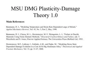
1. MSU DMG Plasticity-Damage Theory 1.0 Main References • Bammann, D. J., "Modeling Temperature and Strain Rate Dependent Large of Metals," Applied Mechanics Reviews, Vol. 43, No. 5, Part 2, May, 1990. Bammann, D. J., Chiesa, M. L., Horstemeyer, M. F., Weingarten, L. I., "Failure in Ductile Materials Using Finite Element Methods," Structural Crashworthiness and Failure, eds. T. Wierzbicki and N. Jones, Elsevier Applied Science, The Universities Press (Belfast) Ltd, 1993. Horstemeyer, M.F., Lathrop, J., Gokhale, A.M., and Dighe, M., “Modeling Stress State Dependent Damage Evolution in a Cast Al-Si-Mg Aluminum Alloy,” Theoretical and Applied Fracture Mechanics, Vol. 33, pp. 31-47, 2000.

2. Background What is a constitutive law? A mathematical description of material behavior to satisfy continuum theory relating stress and strain Number of equations Conservation of mass 1 Balance of linear momentum 3 Balance of angular momentum 3 Balance of energy 1 Number of equations = 8 Number of unknowns=17 Constitutive Law equations =9

3. Restrictions on Constitutive Laws 1. Physical admissibility 2. Material memory 3. Frame indifference 4. Equipresence 5. Local action

4. Physical Admissibility of ISVs ISVs are useful to model collective effects of changing material structure involving multiple mechanisms at multiple length scales e.g. dislocation interactions phase transformations distributed voids/cracks etc. PREMISE: all scales/treatments beyond quantum mechanics arephenomenological to some extent. Degree of “rigor” is related to the degree of resolution selected in solving the problem.

5.  strain stress-strain relation Dislocation Internal State Variable P L 

6. dislocation density

7.  strain stress-strain relation Observable State Variable (strain) Internal State Variable (damage) P L 

8. Internal State Variable (damage) Observable State Variables (strain, strain rate, temperature)

9. Observable State Variables (strain, strain rate, temperature) Internal State Variables (dislocations, damage)

10. Porous Creep-Plastic Material ACTUAL EFFECTIVE CONTINUUM Domain is occupied by dense material and voids/cracks Domain is occupied by voids/cracks Damage is defined by volume fraction or area fraction

11. Porous Creep-Plastic Material ACTUAL EFFECTIVE CONTINUUM Kachanov (1959) Rabotnov (1960)

12. EFFECTIVE CONTINUUM ACTUAL For example, the MSU DMG model,

13. Thermodynamical Framework of MDU DMG 1.0 Internal State Variable Model Elastic and Inelastic parts of Helmholtz Free Energy Stress-strain are thermodynamic conjugates Temperature-entropy are thermodynamic conjugates Backstress-kinematic (anisotropic) hardening are thermodynamic conjugates Global stress-isotropic hardening are thermodynamic conjugates Energy release rate-void volume fraction are thermodynamic conjugates

14. Frost-Ashby deformation mechanism map

15.  Evolution of dislocation density Motivate evolution equations from Kocks-Mecking where dislocation density evolves as a dislocation storage minus recovery event. In an increment of strain dislocations are stored inversely proportional to the mean free path l, which in a Taylor lattice is inversely proportional to the square root of dislocation Density. Dislocations are annihilated or “recover” due to cross slip or climb in a manner proportional to the dislocation density A scalar measure of the stored elastic strain in such a lattice is

16. Temperature Dependent Yield Rather than introducing several flow rules, we propose a temperature dependence for the initial value of the internal strength that emulates all of the mechanisms at a very low strain rate

17. Linear Elasticity Introduce a flow rule of the form From dislocation mechanics, (statistically stored dislocations)

18. Recovery with the Plasticity Constants (Now we have 3 constants: Yield, Isotropic Hardening with recovery) Recovery included for the same compression curve. In this case the model accurately captures both the hardening and recovery through the isotropic hardening variable . Y=C3 H=C15 Rd=C13 STRESS MPa data s  STRAIN

19. Recovery with the Isotropic and Anisotropic Plasticity Constants (Now we have 5 constants: Yield, Isotropic and Kinematic Hardening with recovery) The small strain fit can be improved by including the short transient a which saturates at small strains as a function of its hardening and recovery parameters Y=C3 h=C9 rd=C7 H=C15 Rd=C13

20. Stress State Dependence (Now we have 7 constants: Yield, Isotropic and Kinematic Hardening with recovery and stress state dependence) Y=C3 h=C9 rd=C7 H=C15 Rd=C13 Ca torsion Cb tension/compression

21. High Strain Rate Effects (Now we have 8 constants: Yield, Isotropic and Kinematic Hardening with recovery+ Strain rate dependence on Yield) stress V=C1 Y=C3 h=C9 rd=C7 H=C15 Rd=C13 Ca torsion Cb tension/compression Strain rate 103/sec C1 is the additional stress related to the added strain rate

22. Strain Rate Effects on Static Recovery Creep Effects in Isotropic Hardening (9 constants) Six parameter fit of 304L SS compression data with only the long transient k but including the effects of rate dependence of yield through the parameters V and f . The strain dependent rate effect is captured by the static recovery parameter Rsk in the isotropic hardening. model10[1/s] V=C1 Y=C3 h=C9 rd=C7 H=C15 Rd=C13 Rs=C17 Ca torsion Cb tension/compression model10-1[1/s] k 10[1/s] k 10-1[1/s]

23. Strain Rate Effects on Static Recovery Creep Effects in Isotropic and Kinematic Hardening (10 constants) Seven parameter fit of 304l SS compression curve including the short transient a . This fit will more accurately capture material response during changes in load path direction V=C1 Y=C3 h=C9 rd=C7 rs=C17 H=C15 Rd=C13 Rs=C17 Ca torsion Cb tension/compression

24. Temperature Effects (add even numbers to yield and hardening)

25. Strain rate dependent model correlation Model prediction for 304L stainless steel tension tests or 304L stainless steel is depicted in Figure 1.

26. History is important to predict the future!! 25% wrong answer if history is not considered!! 304L SS

27. Rate and temperature history change Load at 269C, 5200 1/s Reload at 25C .0004 1/s Load at 25C, 6000 1/s Reload at 269C at .0004 1/s

28. Rate change - decreasing at 25C - increasing at 269C

29. Number of ISV Model Constants • 2: Bilinear Hardening • 3: Yield+ Nonlinear Hardening • 5: Yield+Nonlinear Isotropic and Kinematic Hardening • 7: Yield+Nonlinear Isotropic and Kinematic Hardening to distinguish between tension, compression, and torsion • 8: Yield+Nonlinear Isotropic and Kinematic Hardening to distinguish between tension, compression, and torsion to examine high strain rates • 10: Yield+Nonlinear Isotropic and Kinematic Hardening to distinguish between tension, compression, and torsion to examine high strain rates and low rate creep using static recovery • 12: Yield+Nonlinear Isotropic and Kinematic Hardening to distinguish between tension, compression, and torsion to examine high strain rates and low rate creep using static recovery and damage/failure • 23: Yield+Nonlinear Isotropic and Kinematic Hardening to distinguish between tension, compression, and torsion to examine high strain rates and low rate creep using static recovery and damage/failure for temperature dependence • 54: Yield+Nonlinear Isotropic and Kinematic Hardening to distinguish between tension, compression, and torsion to examine high strain rates and low rate creep using static recovery and damage/failure for temperature depedenceincluding all of the nucleation, growth and coalescence for damage/failure

30. 1 2 a 3 1 2 3 Kinematic vs. Isotropic Hardening • If all hardening occurs uniformly by statistically stored dislocations, (and the texture is random), the yield surface would grow isotropically “the same in every direction, independent of the direction of loading”. The radius of the yield surface, is given by k, the internal strength of the material. • This type of loading is illustrated in the figures. The material deforms elastically and the stress increases linearly until the initial yield surface is reached and the material hardens and the yield surface grows until unloading begins at point 1. Upon reversal of load the material deforms elastically until point 3 is reached. • If geometrically necessary dislocations form pileups at grain boundaries (small effect) or at particles (larger effect), the material exhibits an apparent softening upon load reversal • To model this, the yield surface is allowed to translate to the same stress point 1 (red surface). Now upon load reversal, plastic flow begins at point 2. Real material would begin a combination of these two exaggerated figures. This is a short transient and a represents the center of the yield surface. • In some cases, we used to use a as long transient to model texture effects. But now we introduce a structure tensor for this effect. k

31. The evolution of damage is based upon the analytic solution of Cocks and Ashby • Growth of spherical void in a power law creeping material under a three dimensional state of stress • Cocks and Ashby using a bound theorem calculated the approximate growth rate of the void • We utilize the functional form in the evolution of our damage state variable • Failure occurs when a critical level of damage has accumulated and the material becomes unstable

32. Brittle vs. Ductile Fracture A. Very ductile, soft metals (e.g. Pb, Au) at room temperature, other metals, polymers, glasses at high temperature. B. Moderately ductile fracture, typical for ductile metals C. Brittle fracture, cold metals, ceramics.

33. Ductile Fracture (Dislocation Mediated) • Necking • Void Nucleation • Void Coalescence • Void Growth • Fracture (cup and cone)

34. Macroscopic • Prominent necking • “Cup & Cone” fracture face • “Dull” fracture surface • +/-45 shear bands visible on side of neck Ductile Fracture

35. Ductile Fracture • Microscopic • Dimples with inclusions • Inclusions suggest processing problem? • Direction of dimples can indicate load history or misaligned photo • TEM or SEM?

38. Ductile vs Brittile

39. Monotonic Microstructure-Property Model (Macroscale) B C D E A Stress (from highest to lowest) D A C E B Inclusion (from most severe to less severe) B E A D C Damage (from most severe to less severe) A D E C B • Plasticity/Damage Inputs • 21 constants for plasticity determined from different strain rate and temperature tests under compression • 6 constants for void nucleation, void growth, and void coalescence equation determined from torsion, tension, and compression tests • Microstructure-Defect Inputs • Silicon (volume fraction, size distribution, nearest neighbor distance) • Porosity (volume fraction, size distribution, nearest neighbor distance) • Dendrite Cell Size distribution • Other inclusion features (eg, oxides, etc) • Outputs • Time and location of failure on complex geometrical component using FEA • Bauschinger effect • Various strain rate and temperature histories • Various loading path sequences (eg, fatigue followed by tensile loading, etc) • Implemented in ABAQUS finite element code • Future • Addition of chemical corrosion effects

40. Microstructure-Property Model Equations (Macroscale) stress-strain relations Dislocation-plasticity internal state variables Damage internal state variables

41. Kinematics of Damage Framework Multiplicative Decomposition of the deformation gradient Damage definition

42. ˙ ˙ ˙ D   v , D   v   v dV dV dN 1 a 1 a a D    v  v v dV dN dV a 2 2 ˙  v  v   v ˙ ˙ D  , D  a a a 1   v 2 2 2   1   v a a ˙     ˙ ˙ D  1  exp(   v ), D   v   v exp   v 3 a 3 a a a ˙ ˙ ˙ D    v , D    v 4 a 4 a Damage Descriptions Barbee et al. (1972), Davison et al. (1977), etc. Davison et al. (1977) N - total number of nucleation site s V - void volume v Kolmogorov (1937), Avarami (1939), Johnson (1949) Gurson, Needleman, Tvergaard, LeBlond, McDowell, etc.

43. Description of Damage # voids/unit volume measured in intermediate configuration average void volume total volume of voids damage definition damage in terms of nucleation density and void volume and coalescence

44. Philosophy Of Modeling Structural Analysis Steering Knuckle Upper Control Arm Experiments FEM Atomistics Macromechanics Continuum Model Cyclic Plasticity Damage Model Cohesive Energy Critical Stress Experiment Uniaxial Monotonic Torsional Monotonic Notch Tensile Fatigue Crack Growth Cyclic Plasticity Analysis Fracture Interface Debonding FEM Analysis Torsion Compression Tension Monotonic/Cyclic Loads Micromechanics ISV Model Void Nucleation Mesomechanics Experiment Fracture Interface Debonding IVS Model Void Growth Void/Void Coalescence Void/Particle Coalescence ISV Model Void Growth Void/Crack Nucleation Experiment Fracture of Silicon Growth of Holes FEM Analysis Idealized Geometry Realistic Geometry Fem Analysis Idealized Geometry Realistic RVE Geometry Monotonic/Cyclic Loads Crystal Plasticity

45. Evolution of Damage

46. Figure 2.3. The damage model encompasses the limiting cases shown by (a) a single void growing in and (b) just void nucleation.

47. Scales of Importance for A356 Al Control Arm • Electronic Principles (void-crack nucleation) Nm • Gave bi-material elastic interfacial energy and moduli • Atomistic (void-crack nucleaction) Nm • Gave critical stresses for interface debonding • Microscale (void-crack nucleation) 1-20 mm • Gave temperature dependence on void-crack nucleation and microstructural • morphological effects such as particle size, shape, and spacing • Mesoscale I (silicon-porosity interactions) 1-200 mm • Gave coalescence affects of second phase particles with casting porosity • Mesoscale II (pore-pore interactions) 200-500 mm • Gave coalescence effects of casting porosity interactions that considered • void volume fraction, size, shape, and distribution at different temperatures and strain rates • Macroscale (constitutive model formulation) mm-cm • Material model was developed that included lower scale effects of microstructures • that allows analysis of history effects • Structural scale (control arm, etc.) cm-m • Predicted and experimentally verified simulations at structural scale to validate • multiscale methodology

48. Al-Si Atomistic Simulations were used to determine Damage nucleation mechanism

49. Atomistic simulations: An elastic fracture criterion approximates solution fairly accurately

50. Void Nucleation Parametric Study Particle Parameters 1. Size 2. Shape 3. Number density 4. Temperature 5. Prestrain anisotropy 6. Microporosity 7. Loading direction