Download
1 / 60
630 likes | 952 Vues
Lectures 17,18 – Boosting and Additive Trees. Rice ECE697 Farinaz Koushanfar Fall 2006. Summary. Bagging and ensemble learning Boosting – AdaBoost.M1 algorithm Why boosting works Loss functions Data mining procedures Example – spam data. Bagging ( Bootstrap Aggregation).

E N D
Lectures 17,18 – Boosting and Additive Trees Rice ECE697 Farinaz Koushanfar Fall 2006
Summary • Bagging and ensemble learning • Boosting – AdaBoost.M1 algorithm • Why boosting works • Loss functions • Data mining procedures • Example – spam data
Bagging ( Bootstrap Aggregation) • Training set D={(x1,y1),…,(xN,yN)} • Sample S sets of N elements from D (with replacement): D1, D2, …,DS • Train on each Ds, s=1,..,S and obtain a sequence of S outputs f1(X),..,fS(X) • The final classifier is: Regression Classification
Bagging: Variance Reduction • If each classifier has a high variance (unstable) the aggregated classifier has a smaller variance than each single classifier • The bagging classifier is like an approximation of the true average computed by replacing the probability distribution with bootstrap approximation
Measuring Bias and Variance in Practice • Bias and Variance are both defined as expectations: • Bias (X) = EP[f(X)-fbar(X)] • Var(X) = EP[(f(X)-fbar(X))2] • It is easy to see why bagging reduces variance – averaging • Bagging is a simple example of an ensemble learning algorithm • Ensemble learning:combine the prediction of different hypothesis by some sort of voting
Boosting • An ensemble-learning method • One of the most powerful learning ideas introduced in the past 10+ years • A procedure that combines many weak classifiers to produce a powerful committee Example: weak learner T. Jaakkola, MIT
Boosting (Cont’d) • In an ensemble, the output of an instance is computed by averaging the output of several hypothesis • Choose the individual classifiers and their ensembles to get a good fit • Instead of constructing the hypothesis independently, construct them such that new hypothesis focus on instance that were problematic for the previous hypothesis • Boosting implements this idea!
Main Ideas of Boosting • New classifiers should focus on difficult cases • Examine the learning set • Get some “rule of thumb” (weak learner ideas) • Reweight the examples of the training set, concentrate on “hard” cases for the previous rule • Derive the next rule of thumb! • …. • Build a single, accurate predictor by combining the rules of thumb • Challenges: how to reweight? How to combine?
Ada Boost.M1 • The most popular boosting algorithm – Fruend and Schapire (1997) • Consider a two-class problem, output variable coded as Y {-1,+1} • For a predictor variable X, a classifier G(X) produces predictions that are in {-1,+1} • The error rate on the training sample is
Ada Boost.M1 (Cont’d) • Sequentially apply the weak classification to repeatedly modified versions of data • produce a sequence of weak classifiers Gm(x) m=1,2,..,M • The predictions from all classifiers are combined via majority vote to produce the final prediction
Algorithm AdaBoost.M1 Some slides borrowed from http://www.stat.ucl.ac.be/
Example: Adaboost.M1 • The features X1,..,X10 are standard independent Gaussian, the deterministic target is =9.34 is the median of the chi-square RV with 10 DF • 2000 training cases, with approximately 1000 cases in each class and 10,000 test observations • Weak classifier: a two-terminal node tree • The weak classifiers produce around 46% correct guesses
Boosting Fits an Additive Model Source http://www.stat.ucl.ac.be/
Forward Stagewise Additive Modeling • An approximate solution to the minimization problem is obtained via forward stagewise additive modeling (greedy algorithm) Source http://www.stat.ucl.ac.be/
Why adaBoost Works? • Adaboost is a forward stagewise additive algorithm using the loss function Source http://www.stat.ucl.ac.be/
Why Boosting Works? (Cont’d) Source http://www.stat.ucl.ac.be/
Loss Function Source http://www.stat.ucl.ac.be/
Loss Function (Cont’d) Source http://www.stat.ucl.ac.be/
Loss Function (Cont’d) • Y.f(X) is called the Margin • In classifications with 1/-1, margin is just like squared error loss (Y-f(X)) • The classification rule implies that observations with positive margin yif(xi)>0 were classified correctly, but the negative margin ones are incorrect • The decision boundary is given by the f(X)=0 • The loss criterion should penalize the negative margins more heavily than the positive ones
Loss Function (Cont’d) Source http://www.stat.ucl.ac.be/
Loss Functions (Cont’d) Source http://www.stat.ucl.ac.be/
Data Mining Source http://www.stat.ucl.ac.be/
Data Mining (Cont’d) Source http://www.stat.ucl.ac.be/
Spam Data Source http://www.stat.ucl.ac.be/
Trees Reviewed! • Partition of the joint predictor values into disjoint regions Rj, j=1,..,J represented by the terminal nodes • A constant j is assigned to each region, • The predictive rule is: xRjf(x)=j • The tree is: T(x;) = J jI(x Rj) • With parameters {Rj, j}; j=1,…,J • We find the parameters by minimizing the empirical risk
Optimization problem on Trees • Finding j given Rj: this is easy • Finding Rj: this is difficult, we typically approximate. We have talked about the greedy top-down recursive partitioning algorithm • We have previously defined some smoother approximate loss criterion for growing tree that are easier to work with • A boosted tree, is sum of such trees,
Boosting Trees Source http://www.stat.ucl.ac.be/
Boosting Trees (cont’d) • Finding the regions is more difficult than before • For a few cases, the problem might simplify!
Boosting Trees (Cont’d) • For squared error regression, solution is similar to single tree • Find the regression tree than best predicts the current residuals yi-fm-1(xi) and j is the mean of these residuals in each corresponding region • For classification and exponential loss, it is the AdaBoost for boosting trees (scaled trees) • Find the tree that minimizes the weighted error, with weights w(m)i defined as before for boosting
Numerical Optimization • Loss function in using prediction f(x) for y is • The goal is to minimize L(f) w.r.t f, where f is the sum of the trees. Ignoring this, we can view minimizing as a numerical optimization f^=argminf L(f) • Where the parameters f are the values of the approximating function f(xi) at each of the N data points xi: f={f(x1),…,f(xN)}, • Solve it as a sum of component vectors, where f0=h0 is the initial guess and each successive fm is induced based on the current parameter vector fm-1
Steepest Descent • Choose hm= -mgm, where m is a scalar andgm is the gradient of L(f) evaluated at f=fm-1 • The step lengthm is the solution to m=argmin L(fm-1- gm) • The current solution is then updated: fm=fm-1- mgm Source http://www.stat.ucl.ac.be/
Gradient Boosting • Forward stagewise boosting is also a very greedy algorithm • The tree predictions can be thought about like negative gradients • The only difficulty is that the tree components are not independent • Search for tm’s corresponding to {T(xi;m)}for xiRjm • They are constrained to be the predictions of a Jm-terminal node decision tree, whereas the negative gradient is unconstrained steepest descent • Unfortunately, the gradient is only defined at the training data points and is not applicable to generalizing fM(x) to new data • See Table 10.2 for the gradients of commonly used loss functions!
Gradient Boosting Source http://www.stat.ucl.ac.be/
Multiple Additive Regression Trees (MART) Source http://www.stat.ucl.ac.be/
MART (Cont’d) Source http://www.stat.ucl.ac.be/
MART (Cont’d) • Besides the size of each tree J, the other meta parameter of MART is M, the number of boosting iterations • Each iterations reduces the training risk, for M large enough training risk can be made small • May lead to overfitting • Like before, we may need shrinkage!
MART (Cont’d) Source http://www.stat.ucl.ac.be/
Penalized Regression • Consider the set of all possible J-terminal trees ={Tk}, K=|| that is realized on training data as basis functions in p, linear model is • Penalized least square is required, where is a vector of parameters and J() is penalizer! • Since we have a large number of basis functions, solving with lasso is not possible • Algorithm 10.4 is proposed instead