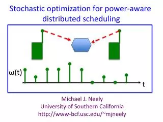
Stochastic optimization for power-aware distributed scheduling
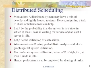
Stochastic optimization for power-aware distributed scheduling. ω (t). t. Michael J. Neely University of Southern California http://www- bcf.usc.edu /~ mjneely. Outline. Lyapunov optimization method Power-aware wireless transmission Basic problem Cache-aware peering

Stochastic optimization for power-aware distributed scheduling
E N D
Presentation Transcript
Stochastic optimization for power-aware distributed scheduling ω(t) t Michael J. Neely University of Southern California http://www-bcf.usc.edu/~mjneely
Outline • Lyapunov optimization method • Power-aware wireless transmission • Basic problem • Cache-aware peering • Quality-aware video streaming • Distributed sensor reporting and correlated scheduling
A single wireless device R(t) = r(P(t), ω(t)) chosen observed Timeslots t = {0, 1, 2, …} ω(t) = Random channel state on slot t P(t) = Power used on slot t R(t) = Transmission rate on slot t (function of P(t), ω(t))
Example R(t) = log(1 + P(t)ω(t)) chosen observed ω(t) t R(t) t
Example R(t) = log(1 + P(t)ω(t)) chosen observed ω(t) t R(t) t
Example R(t) = log(1 + P(t)ω(t)) chosen observed ω(t) t R(t) t
Optimization problem Maximize: R Subject to: P ≤ c • Given: • Pr[ω(t)=ω] = π(ω) , ω in {ω1, ω2, …, ω1000} • p(t) in P = {p1, p2, …, p5} • c = desired power constraint
Consider randomized decisions • ω(t) in {ω1, ω2, …, ω1000} • P(t) in P = {p1, p2, …, p5} Pr[pk| ωi] = Pr[P(t) = pk| ω(t)=ωi] 5 ∑Pr[pk| ωi] = 1 ( for all ωiin {ω1, ω2, …, ω1000} ) k=1
Linear programming approach 5 1000 Max: R S.t. : P ≤ c Max: ∑ ∑ π(ωi)Pr[pk|ωi] r(pk,ωi) i=1 k=1 5 1000 S.t.: ∑ ∑ π(ωi)Pr[pk|ωi] pk ≤ c i=1 k=1 Given parameters: π(ωi) (1000 probabilities) r(pk , ωi) (5*1000 coefficients) Optimization variables: Pr[pk|ωi] (5*1000 variables)
Multi-dimensional problem R1(t) Access Point 1 2 N RN(t) R2(t) • Observe (ω1(t), …, ωN(t)) • Decisions: • -- Choose which user to serve • -- Choose which power to use
Goal and LP approach Maximize: R1 + R2 + … + RN Subject to: Pn ≤ c for all n in {1, …, N} LP has given parameters: π(ω1, …, ωN) (1000N probabilities) rn(pk , ωi) (N*5N*1000N coefficients) LP has optimization variables: Pr[pk|ωi] (5N*1000N variables)
Advantages of LP approach • Solves the problem of interest • LPs have been around for a long time • Many people are comfortable with LPs
Disadvantages of LP approach • Need to estimate an exponential number of probabilities. • LP has exponential number of variables. • What if probabilities change? • Fairness? • Delay? • Channel errors?
Lyapunov optimization approach Maximize: R1 + R2 + … + RN Subject to: Pn ≤ c for all n in {1, …, N}
Lyapunov optimization approach Maximize: R1 + R2 + … + RN Subject to: Pn ≤ c for all n in {1, …, N} • Virtual queue for each constraint: • Stabilizing virtual queue constraint satisfied! Qn(t) Pn(t) c Qn(t+1) = max[Qn(t) + Pn(t) – c, 0]
Lyapunov drift Q2 Q1 L(t) = ½ ∑Qn(t)2 Δ(t) = L(t+1) – L(t) n
Drift-plus-penalty algorithm • Every slot t: • Observe (Q1(t), …., QN(t)), (ω1(t), …, ωN(t)) • Choose (P1(t), …, PN(t)) to greedily minimize: • Update queues. Δ(t) - (1/ε)(R1(t) + … + RN(t)) drift penalty Low complexity No knowledge of π(ω) probabilities is required
Specific DPP implementation • Each user n observes ωn(t), Qn(t). • Each user n chooses Pn(t) in P to minimize: • -(1/ε)rn(Pn(t), ωn(t)) + Qn(t)Pn(t) • Choose user n* with smallest such value. • User n* transmits with power level Pn*(t). Low complexity No knowledge of π(ω) probabilities is required
Performance Theorem • Assume it is possible to satisfy the constraints. Then under DPP with any ε>0: • All power constraints are satisfied. • Average thruput satisfies: • Average queue size satisfies: • ∑Qn ≤ O(1/ε) R1 + … + RN ≥ throughputopt – O(ε)
General SNO problem ω(t) = Observed random event on slot t π(ω) = Pr[ω(t)=ω] (possibly unknown) α(t) = Control action on slot t Aω(t)= Abstract set of action options Minimize: y0(α(t), ω(t)) Subject to: yn(α(t), ω(t)) ≤ 0 for all n in {1, …, N} α(t) in Aω(t) for all t in {0, 1, 2, …} Such problems are solved by the DPP algorithm. Performance theorem: O(ε), O(1/ε) tradeoff.
What we have done so far • Lyapunov optimization method • Power-aware wireless transmission • Basic problem • Cache-aware peering • Quality-aware video streaming • Distributed sensor reporting and correlated scheduling
What we have done so far • Lyapunov optimization method • Power-aware wireless transmission • Basic problem • Cache-aware peering • Quality-aware video streaming • Distributed sensor reporting and correlated scheduling
What we have done so far • Lyapunov optimization method • Power-aware wireless transmission • Basic problem • Cache-aware peering • Quality-aware video streaming • Distributed sensor reporting and correlated scheduling
What we have done so far • Lyapunov optimization method • Power-aware wireless transmission • Basic problem • Cache-aware peering • Quality-aware video streaming • Distributed sensor reporting and correlated scheduling
Mobile P2P video downloads Access Point
Mobile P2P video downloads Access Point
Mobile P2P video downloads Access Point
Mobile P2P video downloads Access Point Access Point
Mobile P2P video downloads Access Point Access Point Access Point
Mobile P2P video downloads Access Point Access Point Access Point
Mobile P2P video downloads Access Point Access Point Access Point
Mobile P2P video downloads Access Point Access Point Access Point
Mobile P2P video downloads Access Point Access Point Access Point
Mobile P2P video downloads Access Point Access Point Access Point
Cache-aware scheduling • Access points (including “femto” nodes) • Typically stationary • Typically have many files cached • Users • Typically mobile • Typically have fewer files cached • Assume each user wants one “long” file • Can opportunistically grab packets from any nearby user or access point that has the file.
Quality-aware video delivery Quality Layer L Bits: 419640 D: 0 Bits: 299216 D: 0 Bits: 277256 D: 0 Bits: 40968 D: 0 Quality Layer 2 Bits: 7370 D: 10.777 Bits: 59984 D: 6.129 Bits: 41304 D: 6.716 Bits: 72800 D: 6.261 Quality Layer 1 Bits: 8176 D: 11.045 Bits: 97864 D: 6.971 Bits: 58152 D: 7.363 Bits: 120776 D: 7.108 Video chunks as time progresses • D = Distortion. • Results hold for any matrices Bits(layer, chunk), D(layer, chunk). • Bits are queued for wireless transmission.
Fair video quality delivery Minimize: f( D1 ) + f( D2 ) + … + f( DN ) Subject to: Pn ≤ c for all n in {1, …, N} Video playback rate constraints
Fair video quality delivery Minimize: f( D1 ) + f( D2 ) + … + f( DN ) Subject to: Pn ≤ c for all n in {1, …, N} Video playback rate constraints Recall the general form: Min: y0 S.t. : yn ≤ 0 for all n α(t) in Aω(t) for all t
Fair video quality delivery Minimize: f( D1 ) + f( D2 ) + … + f( DN ) Subject to: Pn ≤ c for all n in {1, …, N} Video playback rate constraints Recall the general form: Min: y0 S.t. : yn ≤ 0 for all n α(t) in Aω(t) for all t Define Yn(t) = Pn(t) - c
Fair video quality delivery Minimize: f( D1 ) + f( D2 ) + … + f( DN ) Subject to: Pn ≤ c for all n in {1, …, N} Video playback rate constraints Recall the general form: Min: y0 S.t. : yn ≤ 0 for all n α(t) in Aω(t) for all t Define auxiliary variable γ(t) in [0, Dmax]
Equivalence via Jensen’s inequality Minimize: f( D1 ) + f( D2 ) + … + f( DN ) Subject to: Pn ≤ c for all n in {1, …, N} Video playback rate constraints Minimize: f( γ1(t)) + f( γ2(t)) + … + f( γN(t)) Subject to: Pn ≤ c for all n in {1, …, N} γn = Dn for all n in {1, …, N} Video playback rate constraints
Example simulation • Region dividedinto 20 x 20 subcells • (only a portion shown here). • 1250 mobile devices, 1 base station • 3.125 mobiles/subcell BS
Phases 1, 2, 3: File availability prob = 5%, 10%, 7% • Basestation Average Traffic: 2.0 packets/slot • Peer-to-Peer Average Traffic: 153.7 packets/slot • Factor of 77.8 gain compared to BS alone!
What we have done so far • Lyapunov optimization method • Power-aware wireless transmission • Basic problem • Cache-aware peering • Quality-aware video streaming • Distributed sensor reporting and correlated scheduling
Distributed sensor reports ω1(t) 1 Fusion Center ω2(t) 2 • ωi(t) = 0/1 if sensor i observes the event on slot t • Pi(t) = 0/1 if sensor i reports on slot t • Utility: U(t) = min[P1(t)ω1(t) + (1/2)P2(t)ω2(t),1] Maximize: U Subject to: P1 ≤ c P2 ≤ c
What is optimal? Agree on plan t 0 1 2 4 3
What is optimal? Agree on plan t 0 1 2 4 3 • Example plan: • User 1: • t=even Do not report. • t=odd Report if ω1(t)=1. • User 2: • t=even Report if ω2(t)=1 • t=odd: Report with prob ½ if ω2(t)=1