Download

1 / 82
820 likes | 854 Vues
Explore the development of low jet noise aircraft engines using advanced Computational Aeroacoustics (CAA) methodology, Large Eddy Simulation (LES), and numerical methods for jet aeroacoustics research. Findings reveal a stable dynamic subgrid-scale model for jet flows, accurate comparison with experimental results, and a promising outlook for future noise reduction endeavors.

E N D
Development of Low Jet Noise Aircraft Engines Anastasios Lyrintzis School of Aeronautics & Astronautics Purdue University
Acknowledgements • Indiana 21st Century Research and Technology Fund • Prof. Gregory Blaisdell • Rolls-Royce, Indianapolis (W. Dalton, Shaym Neerarambam) • L. Garrison, C. Wright, A. Uzun, P-T. Lew
Motivation • Airport noise regulations are becoming stricter. • Jet exhaust noise is a major component of aircraft engine noise • Lobe mixer geometry has an effect on the jet noise that needs to be investigated.
Methodology • 3-D Large Eddy Simulation for Jet Aeroacoustics • RANS for Forced Mixers • Coupling between LES and RANS solutions • Semi-empirical method • (Experiments at NASA Glenn)
Objective • Development and full validation of a Computational Aeroacoustics (CAA) methodology for jet noise prediction using: • A 3-D Large Eddy Simulation (LES) code working on generalized curvilinear grids that provides time-accurate unsteady flow field data • A surface integral acoustics method using LES data for far-field noise computations
Numerical Methods for LES • 3-D Navier-Stokes equations • 6th-order accurate compact differencing scheme for spatial derivatives • 6th-order spatial filtering for eliminating instabilities from unresolved scales and mesh non-uniformities • 4th-order Runge-Kutta time integration • Localized dynamic Smagorinsky subgrid-scale (SGS) model for unresolved scales
Computational Jet Noise Research • Some of the biggest jet noise computations: • Freund’s DNS for ReD = 3600, Mach 0.9 cold jet using 25.6 million grid points (1999) • Bogey and Bailly’s LES for ReD = 400,000, Mach 0.9 isothermal jets using 12.5 and 16.6 million grid points (2002, 2003) • We studied a Mach 0.9 turbulent isothermal round jet at a Reynolds number of 100,000 • 12 million grid points used in our LES
Computation Details • Physical domain length of 60ro in streamwise direction • Domain width and height are 40ro • 470x160x160 (12 million) grid points • Coarsest grid resolution: 170 times the local Kolmogorov length scale • One month of run time on an IBM-SP using 160 processors to run 170,000 time steps • Can do the same simulation on the Compaq Alphaserver Cluster at Pittsburgh Supercomputing Center in 10 days
Mean Flow Results • Our mean flow results are compared with: • Experiments of Zaman for initially compressible jets (1998) • Experiment of Hussein et al. (1994) Incompressible round jet at ReD = 95,500 • Experiment of Panchapakesan et al. (1993) Incompressible round jet at ReD = 11,000
Jet Aeroacoustics • Noise sources located at the end of potential core • Far field noise is estimated by coupling near field LES data with the Ffowcs Williams–Hawkings (FWH) method • Overall sound pressure level values are computed along an arc located at 60ro from the jet nozzle • Cut-off Strouhal number based on grid resolution is around 1.0
Jet Aeroacoustics (continued) • OASPL results are compared with: • Experiment of Mollo-Christensen et al. (1964) Mach 0.9 round jet at ReD = 540,000 (cold jet) • Experiment of Lush (1971) Mach 0.88 round jet at ReD = 500,000 (cold jet) • Experiment of Stromberg et al. (1980) Mach 0.9 round jet at ReD =3,600 (cold jet) • SAE ARP 876C database
Conclusions • Localized dynamic SGS model stable and robust for the jet flows we are studying • Very good comparison of mean flow results with experiments • Aeroacoustics results are encouraging • Valuable evidence towards the full validation of our CAA methodology has been obtained
Near Future Work • Simulate Bogey and Bailly’s ReD = 400,000 jet test case using 16 million grid points • 100,000 time steps to run • About 150 hours of run time on the Pittsburgh cluster using 200 processors • Evaluate noise sources (Tij) • Do a more detailed study of surface integral acoustics methods
Can a realistic LES be done for ReD = 1,000,000 ? • Assuming 50 million grid points provide sufficient resolution: • 200,000 time steps to run • 30 days of computing time on the Pittsburgh cluster using 256 processors • Only 3 days on a near-future computer that is 10 times faster than the Pittsburgh cluster
Future Work • Extend methodology to handle: • Noise from unresolved scales • Supersonic flow • Solid boundaries (nozzle lips) • Complicated (mixer) geometries multi-block code
Objective • Use RANS to study flow characteristics of various flow shapes
Nozzle Bypass Flow Mixer Exhaust Flow Core Flow Tail Cone Lobed Mixer Mixing Layer Exhaust / Ambient Mixing Layer Internally Forced Mixed Jet
Forced Mixer H H: Lobe Penetration (Lobe Height)
2nd order upwind scheme 1.7 million/7 million grid points 8-16 zones 8-16 LINUX processors Spalart-Allmaras/ SST turbulence model Wall functions WIND Code options
Grid Dependence Density Contours 1.7 million grid points Density Contours 7 million grid points
Grid Dependence 1.7 million grid points 7 million grid points Density Vorticity Magnitude
Spalart-Allmaras and Menter SST Turbulence Models Spalart-Allmaras Menter SST
Spalart-Allmaras and and Menter SST at Nozzle Exit Plane SST Spalart Density Vorticity Magnitude
Mean Axial Velocity at x = 2.88”(High Penetration) Spalart Allmaras ¼ Scale Spalart at x = 2.88/4” experiment
Mean Axial Velocity at x = 2.88”(High Penetration) ¼ Scale Menter SST at x = 2.88/4” experiment Menter SST
Spalart-Allmaras vs. Menter SST • The Spalart-Allmaras model appears to be less dissipative. The vortex structure is sharper and the vorticity magnitude is higher at the nozzle exit. • The Menter SST model appears to match experiments better, but the experimental grid is rather coarse and some of the finer flow structure may have been effectively filtered out. • Still unclear which model is superior. No need to make a firm decision until several additional geometries are obtained.
Geometry at Mixer Exit Low Penetration Mid Penetration High Penetration