Link State Routing
Link State Routing. Using Link Cost as a Metric. Link State Routing. Also called shortest path first (SPF) forwarding Named after Dijkstra’s algorithm (1959) which it uses to compute routes All routers have tables which contain a representation of the entire network topology

Link State Routing
E N D
Presentation Transcript
Link State Routing Using Link Cost as a Metric
Link State Routing • Also called shortest path first (SPF) forwarding • Named after Dijkstra’s algorithm (1959) which it uses to compute routes • All routers have tables which contain a representation of the entire network topology • In the form of lists of routers and information about each router’s neighbours and the connection between the two
Link State Routing • Each router creates a link state packet (LSP) which contains names (e.g. network addresses) and cost to each of its neighbours • The LSP is transmitted to all other routers, who each update their own records • When a routers receives LSPs from all routers, it can use (collectively) that information to make topology-level decisions
Link State Packets • LSPs are generated and distributed when: • A time period passes • New neighbours connect to the router • The link cost of a neighbour has changed • A link to a neighbour has failed (link failure) • A neighbour has failed (node failure)
Link State Packets • LSP are essentially a list of tuples, containing: • The name of a neighbour to a router • Which may be a router or a network • The cost of the link to that neighbour
Link State Packets • Distribution of LSPs can be difficult • Routers themselves are the means for delivering messages • How do routers deliver their own messages, particularly when routers are in an inconsistent state • e.g. During link failure, before each router has been notified of the problem
Link State Packets • One method for LSP distribution: Flooding • Each LSP received is transmitted to every direct neighbour (except the neighbour where the LSP came from) • This creates an exponential number of packets on the network (similar to O(2R), where R is the number of routers) • It does, however, guarantee that the LSP will be received by every router • Assuming that node or link failure does not occur, and LSPs are not somehow lost
Link State Packets • An improvement on this scheme is as follows: • When an LSP is received, it is compared with the stored copy • If it is identical to the stored copy, it is dropped • If it is different, the stored LSP is overwritten with the new LSP and the LSP is transmitted to every direct neighbour (except the source of the LSP) • This scheme works because if a given router has already received a LSP from another neighbour, it will have also already distributed the LSP to all of its neighbours • This scheme has a network complexity similar to O(R2)
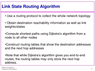
Link State Routing Algorithm • Ok, now that we know how to distribute LSPs, how are they used to determine routes? • The algorithm used (mostly) was developed by Dijkstra • Essentially, the algorithm runs at each router, computing each possible path to the destination, adding up each cost • The path with the lowest cost is used
Link State Routing Algorithm • The algorithm requires the following information: • Link state database: List of all the latest LSPs from each router on the network • Path: Tree structure storing previously computed best paths • Consider this a sort of cache • Data type for nodes: (ID, path cost, port) • Tent: Tree structure storing paths currently being tested and compared (tentative) • Consider this a sort of rough workspace • Data type for nodes: (ID, path cost, port) • Forwarding database: Table storing all IDs that can be reached, and the port to which messages should be sent • This is simply a reduced version of the ‘Path’, which contains (destination,port) pairs • This can be used by the router to quickly forward packets for which the best path has already been determined • Data type for table rows: (ID, port)
Dijkstra’s LSR Algorithm • Initially, PATH is just a root containing (this router’s ID, 0, 0) • For every node placed into path, N: • For all neighbours M of node N: • If M is not in TENT, add a node to TENT for M (use the LSP for N to determine link cost) • If M is in TENT already, and its cost is lower than an existing entry for M, replace that entry with information from N’s LSP • If M is in TENT already, but its cost is higher, ignore N’s link to M • Calculate the shortest route in TENT • If the shortest route has lower cost than the route in PATH, overwrite the route in PATH with the route in TENT
Dijkstra’s LSR Algorithm • Consider the following network: 6 2 A B C 5 2 1 2 G 2 4 D E F 1 Link state database:
Dijkstra’s LSR Algorithm • Now, if we want to generate a PATH for C: • First, we add (C,0,0) to PATH C (0)
Dijkstra’s LSR Algorithm • Examine C’s LSP • Add F, G, and B to TENT C (0) (2) (5) (2) F G B
Dijkstra’s LSR Algorithm • Place F in PATH (shown as solid line) • Add G and E to TENT (adding costs) C (0) (2) (5) (2) F G B (3) (6) G E
Dijkstra’s LSR Algorithm • G exists in TENT twice, keep only the best • The new G is a better path than the old (3 < 5) C (0) (2) (5) (2) F G B (3) (6) G E
Dijkstra’s LSR Algorithm • Put B into path (shown as solid line) • Add A and E to TENT C (0) (2) (2) F B (3) (6) (3) (8) G A E E
Dijkstra’s LSR Algorithm • E exists in TENT twice, keep only the best • The new E is better than the old (3 < 6) C (0) (2) (2) F B (3) (6) (3) (8) G A E E
Dijkstra’s LSR Algorithm • Place E in PATH (shown as solid line) • Add D to TENT C (0) (2) (2) F B (3) (3) (8) G A E (5) D
Dijkstra’s LSR Algorithm • Place G in PATH (shown as solid line) • All G’s LSP elements already exist in TENT C (0) (2) (2) F B (3) (3) (8) G A E (5) D
Dijkstra’s LSR Algorithm • Place D in PATH (shown as solid line) • Add path to A since it is better than old A C (0) (2) (2) F B (3) (3) (8) G A E (5) D (7) A
Dijkstra’s LSR Algorithm • Place A in PATH (shown as solid line) • All A’s LSP elements already exist in PATH C (0) (2) (2) F B (3) (3) G E (5) D (7) A
Dijkstra’s LSR Algorithm • We are done since all routes from TENT were placed into PATH C (0) (2) (2) F B (3) (3) G E (5) D (7) A
Dijkstra’s LSR Algorithm • We can now create a forwarding database: C (0) (2) (2) F B (3) (3) G E (5) D (7) A
LSR Topology Changes • LSR forwarding tables must be recalculated whenever a topology change occurs • For example, a new router and/or link is added to the network • This new link may provide a more efficient route to one or more other nodes • For example, a given link’s cost is reduced • This new link may now provide the lowest total cost route to a destination that was previously forwarded in another direction • For example, a given link’s cost is increased • This new link may no longer provide the lowest total cost route to a given destination, and another route should now be chosen
LSR Topology Changes • In a nutshell, LSR routers should invalidate (indicate that it needs to be regenerated) its PATH data structure, and thus its forwarding table • The entire PATH generation algorithm (e.g. Dijkstra’s algorithm) should be reapplied
Topology Change Example • Let’s consider our previously generated PATH structure for the router C C (0) (2) (2) F B (3) (3) G E (5) D (7) A
Topology Change Example • Say we receive an LSP from router B, indicating the link cost from B to E is now 6 C (0) (2) (2) F B (3) (3) G E (5) D (7) A
Topology Change Example • The total route costs are different in PATH: C (0) (2) (2) F B (3) (8) G E (10) D (12) A
Topology Change Example • Consider for now, only the cost to A C (0) (2) (2) F B (3) (8) G E (10) D (12) A
Topology Change Example • Recall that another path to A existed • Now, that path is more efficient C (0) (2) (2) F B (3) (8) G (8) A E (10) D (12) A
Topology Change Example • The PATH data structure is complete, the forwarding table can now be regenerated C (0) (2) (2) F B (3) (8) G (8) A E (10) D
Topology Change Example • In a router, which will be running as a computer program, finding if a new path exists essentially requires complete re-execution of Dijkstra’s algorithm • For example, there could have been many routes to A, each of which would have to be compared to find the most efficient route
OSPF • Open SPF protocol • SPF: Shortest path first • Essentially the OSPF specification is one specification describing an algorithm implementing shortest path forwarding • It is open, meaning anyone can implement the specification at no cost • Since OSPF is a link state routing (LSR) protocol, it can have load balancing • However, to be deployed on large-scale WANs, the LSP propagation must be limited • OSPF partitions networks into regions called ‘areas’ which contain a subset of the routers • This is similar to schemes used in other LSR protocols
OSPF Autonomous Systems • An OSPF AS allows a multi-level routing strategy to be employed • The complete system is partitioned into autonomous systems (AS) • Within each AS, OSPF routing is used • In this way, the limitation of the number of routers in link state routing is not a factor • Messaging between AS can use ATM
OSPF Messages • There are 5 types of messages in OSPF: • Hello messages • Allow routers to test if a node is reachable • Link State Advertisement (LSA) • Topology information from a router (i.e. LSPs) • Link status request (LSR) • Requests send to another router to determine the status of one or more links • Link status update (LSU) • Responses to a link status request message • Link status acknowledgement • Used to indicate that the LSU was received (reliable transfer)
OSPF Hello Packets • When a router wants to test if a node is reachable, it sends a Hello packet • If the node is reachable, it will respond with its own Hello packet • Hello packets contain a list of reachable addresses (among other things) • A router might query the node about one of those addresses • The node will respond with topology (connectivity) information about the host at that address • In the form of an LSA
OSPF LSA Packets • When requested, these packets contain a list of links (forming a complete route) to a destination • This can be used (including the link cost information) to determine the ‘shortest’ path
OSPF Link Status Requests • This packet represents a request for information about one or more links • A router may be given this request if another router has outdated information
OSPF Link Status Updates • This is a response to a link status request • It contains information about each link requested • Most importantly: the length (cost) of the link
Multicast Routing in OSPF • In OSPF and other link state implementations, multicast routing is supported • For a multicast message, Dijkstra’s path tree is also created • However, in this case, the sender is the root of the tree, not the current router • The current router sends the message to all of its direct child nodes in the tree
PNNI Switches • Used in ATM switches • PNNI is a link state algorithm used for ATM switching • PNNI is multi-level routing • Areas are called peer groups • Peer groups can be arbitrarily connected • Despite the fact that ATM networks are connection-oriented, the process of finding a route for packets/cells is the same • Thus PNNI switching is very similar to OSPF and IS-IS routing
LSR and Load Balancing • At least one scheme for load balancing is possible with LSR: • Multiple routes could be calculated for each destination • As a result, the forwarding table would contain more than one entry for nodes • This technique is known as load splitting
LSR and Load Splitting • Since the forwarding table contains more than one entry for each destination, some scheme must be used to choose one of the entries for each incoming packet • Each entry could have its turn (in a round-robin fashion) • This evenly distributes packets among the different routes • Randomly choose one of the forwarding entries • Use one of the above schemes, but use some preference method to ensure the entry which has more congestion on its link is used less often • Have routers keep an on-going database of link congestion, allowing it to choose the least congested link for each packet (which may change from one packet to another)
LSR and Load Splitting • Advantages • Distributing network load among different routes directly results in more optimal use of network bandwidth • i.e. Network capacity is increased • Disadvantages • The number of out-of-order packets is increased when load splitting is employed • Network delivery times are difficult to estimate • As is frequently important with streaming data (such as streaming audio) where Quality of Service (QoS) is important
LSR and Load Balancing • LSR provides another, more natural, scheme for load balancing • When links become too saturated with packets, alternate routes can be used • For example, a link could be assigned a higher cost due to the amount of traffic • The higher cost could ensure that some of the routers use alternate routes for forwarding
LSR and Load Balancing • The other scheme, varying the link cost as network traffic changes, is another interesting idea • Increasing the link cost as traffic through that link increases allows automatic load balancing to occur • Similarly, link cost can be lowered as traffic through the link decreases • This technique is called ‘variable link cost load balancing’
Variable Link Cost LB • Advantages • The automatic load balancing that results would offer similar improvement in network capacity as when explicitly employing load splitting • Disadvantages • Having link cost change with network congestion results in a need for LSP propagation whenever a significant change in network congestion occurs • As a result, there are more LSPs required than when only network topology changes should force them • Network topology changes happen very rarely, but network congestion varies often • By the time a link cost change is propagated to all routers in the network, the network congestion may have (again) changed
LSR vs. DVR • Bandwidth used by each: • This is dependent upon network topology • Some networks use less bandwidth for LSR than DVR (and vice versa) • Computation used by each: • LSR (Dijkstra): O(n*k*log n) • n: number of nodes on the network • k: average number of links per node • Therefore, n*k is the total number of links • DVR: O(n * k) • However, sometimes the list of distance vectors (n*k of them) must be scanned more than once • It should be fairly obvious that LSR uses more computation than DVR