Chapter 6. Point Estimation
Chapter 6. Point Estimation. Weiqi Luo ( 骆伟祺 ) School of Software Sun Yat-Sen University Email : weiqi.luo@yahoo.com Office : # A313. Chapter 6: Point Estimation. 6.1. Some General Concepts of Point Estimation 6.2. Methods of Point Estimation.

Chapter 6. Point Estimation
E N D
Presentation Transcript
Chapter 6. Point Estimation Weiqi Luo (骆伟祺) School of Software Sun Yat-Sen University Email:weiqi.luo@yahoo.com Office:# A313
Chapter 6: Point Estimation • 6.1. Some General Concepts of Point Estimation • 6.2. Methods of Point Estimation
6.1 Some General Concepts of Point Estimation • In ordert to get some population characteristics, statistical inference needs obtain sample data from the population under study, and achieve the conclusions can then be based on the computed values of various sample quantities (statistics). • Typically, we will use the Greek letter θ for the parameter of interest. The objective of point estimation is to select a single number, based on sample data (statistic ), that represents a sensible value for θ.
6.1 Some General Concepts of Point Estimation • Point Estimation A point estimate of a parameter θ is a single number that can be regarded as a sensible value for θ. A point estimate is obtained by selecting a suitable statistic and computing its value from the given sample data. The selected statistic is called the point estimatorof θ. Here, the type of population under study is usually known, while the paprameters are unkown. A function (statistic ) Population Q #1: How to get the candiate estimators based on the population? A Sample A quantity Parameters θ Q #2: How to measure the candidate estimators? Estimating
estimator estimate = 6.1 Some General Concepts of Point Estimation • Example 6.1 The manufacturer has used this bumper in a sequence of 25 controlled crashes against a wall, each at 10 mph, using one of its compact car models. Let X = the number of crashes that result in no visible damage to the automobile. What is a sensible estimate of the parameter p = the proportion of all such crashes that result in no damage If X is observed to be x = 15, the most reasonable estimator and estimate are
6.1 Some General Concepts of Point Estimation • Example 6.2 Reconsider the accompanying 20 observations on dielectric breakdown voltage for pieces of epoxy resin first introduced in Example 4.29 (pp. 193) The pattern in the normal probability plot given there is quite straight, so we now assume that the distribution of breakdown voltage is normal with mean value μ. Because normal distribution are symmetric, μ is also the median lifetime of the distribution. The given observation are then assumed to be the result of a random sample X1, X2, …, X20 from this normal distribution.
a. Estimator= , estimate= b. Estimator= , estimate= d. Estimator = , the 10% trimmed mean (discard the smallest and largest 10% of the sample and then average) 6.1 Some General Concepts of Point Estimation • Example 6.2 (Cont’) Consider the following estimators and resulting estimates for μ c. Estimator [ min(Xi) + max(Xj)]/2 = the average of the two extreme lifetimes, estimate=[ min(xi)+max(xi)]/2 = (24.46+30.88)/2 = 27.670
6.1 Some General Concepts of Point Estimation • Example 6.3 In the near future there will be increasing interest in developing low-cost Mg-based alloys for various casting processes. It is therefore important to have practical ways of determining various mechanical properties of such alloys. Assume that the observations of a random sample X1, X2, …, X8 from the population distribution of elastic modulus under such circumstances. We want to estimate the population variance σ2 Method #1: sample variance Method #2: Divided by n rather than n-1
+ error of estimation 6.1 Some General Concepts of Point Estimation • Estimation Error Analysis Note that is a function of the sample Xi’s, so it is a random variable. Therefore, an accurate estimator would be one resulting in small estimation errors, so that estimated values will be near the true value θ (unkown). A good estimator should have the two properties: 1. unbiasedness (i.e. the average error should be zero) 2. minimum variance (i.e. the variance of error should be samll)
pdf of pdf of 6.1 Some General Concepts of Point Estimation • Unbiased Estimator A point estimator is said to be an unbiased estimator of θ if for every possible value of θ. If is not unbiased, the difference is called the biasof Note: “centered” here means the expected vaule, not the median, of the the distribution of is equal to θ θ Bias of θ1
6.1 Some General Concepts of Point Estimation • Proposition When X is a binomial rv with parameters n and p, the sample proportion =X/n is an unbiased estimator of p. Refer to Example 6.1, the sample proportion X/n was used as an estimator of p, where X, the number of sample successes, had a binomial distribution with parameters n and p, thus
6.1 Some General Concepts of Point Estimation • Example 6.4 Suppose that X, the reaction time to a certain stimulus, has a uniform distribution on the interval from 0 to an unknown upper limit θ. It is desired to estimate θ on the basis of a random sample X1, X2, …, Xn of reaction times. Since θ is the largest possible time in the entire population of reaction times, consider as a first estimator the largest sample reaction time: Since (refer to Ex. 32 in pp. 279 ) Another estimator biased estimator, why? unbiased estimator
6.1 Some General Concepts of Point Estimation • Proposition Let X1, X2, …, Xn be a random sample from a distribution with mean μ and variance σ2. Then the estimator is an unbiased estimator of σ2 , namely Refer to pp. 259 for the proof. However,
6.1 Some General Concepts of Point Estimation • Proposition If X1, X2,…Xn is a random sample from a distribution with mean μ, then is an unbiased estimator of μ. If in addition the distribution is continuous and symmetric, then and any trimmed mean are also unbiased estimator of μ Refer to the estimators in Example 6.2
pdf of , another unbiased estimator pdf of , an unbiased estimator 6.1 Some General Concepts of Point Estimation • Estimators with Minimum Variance Obivously, the estimator is better than the in this example θ
6.1 Some General Concepts of Point Estimation • Example 6.5 (Ex. 6.4 Cont’) When X1, X2, … Xn is a random sample from a uniform distribution on [0, θ], the estimator is unbiased for θ It is also shown that is the MVUE of θ.
6.1 Some General Concepts of Point Estimation • Theorem Let X1, X2, …, Xn be a random sample from a normal distribution with parameters μ and δ. Then the estimator is the MVUE for μ. How about those un-normal distributions?
pdf of , the MVUE pdf of , a biased estimator 6.1 Some General Concepts of Point Estimation • Estimator Selection • When choosing among several different estimators of θ, select one that is unbiased. • Among all estimators of θ that are unbiased, choose the one that has minimum variance. The resulting is called the minimum variance unbiased estimator (MVUE) of θ. In some cases, a biased estimator is perferable to the MVUE θ
6.1 Some General Concepts of Point Estimation • Example 6.6 Suppose we wish to estimate the thermal conductivity μ of a certain material. We will obtain a random sample X1, X2, …, Xn of n thermal conductivity measurements. Let’s assume that the population distribution is a member of one of the following three families: Gaussian Distribution Cauchy Distribution Uniform Distribution
6.1 Some General Concepts of Point Estimation 1. If the random sample comes from a normal distribution, then is the best of the four estimators, since it is the MVUE. 2. If the random sample comes from a Cauchy distribution, then and (the average of the two extreme observations) are terrible estimators for μ, whereas is quite good; is bad because it is very sensitive to outlying observations, and the heavy tails of the Cauchy distribution make a few such observation likely to appear in any sample. 3. If the underlying distribution is uniform, the best estimator is ; this estimator is greatly influenced by outlying observations, but the lack of tails makes such observations impossible. 4. The trimmed mean is best in none of these three situations, but works reasonably well in all three. That is, does not suffer too much in any of the three situations. A Robust estimator
6.1 Some General Concepts of Point Estimation • The Standard Error The standard error of an estimator is its standard deviation . If the standard error itself involves unknown parameters whose values can be estimated, substitution of these estimates into yields the estimated standard error (estimated standard deviation) of the estimator. The estimated standard error can be denoted either by or by .
6.1 Some General Concepts of Point Estimation • Example 6.8 Assuming that breakdown voltage is normally distributed, is the best estimator of μ. If the value of σ is known to be 1.5, the standard error of is If, as is usually the case, the value of σ is unknown, the estimate is substituted into to obtain the estimated standard error
6.1 Some General Concepts of Point Estimation • Homework Ex. 1, Ex. 8, Ex. 9, Ex. 13
6.2 Methods of Point Estimation • Two “constructive” methods for obtaining point estimators • Method of Moments • Maximum Likehood Estimation
6.2 Methods of Point Estimation • Moments Let X1, X2,…, Xn be a random sample from a pmf or pdf f(x). For k = 1, 2, 3, …, the kth population moment, or kth moment of the distributionf(x),is .The kth sample momentis .
6.2 Methods of Point Estimation • Moment Estimator Let X1, X2, …, Xn be a random sample from a distribution with pmf or pdf f(x;θ1,…,θm), where θ1,…,θm are parameters whose values are unknown. Then the moment estimators are obtained by equating the first msample moments to the corresponding first mpopulation moments and solving for θ1,…,θm . n is large With the given sample xi With unkonwn θi K-th sample moment K-th population moment
6.2 Methods of Point Estimation General Algorithm : The solution of equations The first m population moments Use the first m sample moment to represent the population moments μl
6.2 Methods of Point Estimation • Example 6.11 Let X1, X2, …, Xnrepresent a random sample of service times of n customers at a certain facility, where the underlying distribution is assumed exponential with parameter λ. How to estimate λ by using the method of moments? Step #1: The 1st population moment E(X) = 1/λ then we have λ = 1/ E(X) Step #2: Use the 1st sample moment to represent 1st poulation moment E(X), and get the estimator
6.2 Methods of Point Estimation • Example 6.12 Let X1, …, Xnbe a random sample from a gamma distribution with parameters α and β. Its pdf is There are two parameter need to be estimated, thus, consider the first two monents
6.2 Methods of Point Estimation • Example 6.12 (Cont’) Step #1: Step #2:
6.2 Methods of Point Estimation • Example 6.13 Let X1, …, Xnbe a random sample from a generalized negative binomial distribution with parameters r and p. Its pmf is Determine the moment estimators of parameters r and p. Note: There are two parameters needs to estimate, thus the first two moments are considered.
6.2 Methods of Point Estimation • Example 6.13 (Cont’) Step #1: Step #2:
6.2 Methods of Point Estimation • Maximum Likelihood Estimation (Basic Idea) Experiment: We firstly randomly choose a box, And then randomly choose a ball. Q: If we get a white ball, which box has the Maximum Likelihood being chosen? Box 1 Box 2
6.2 Methods of Point Estimation • Maximum Likelihood Estimation (Basic Idea) Q: What is the probability p of hitting the target? … The best one among the four options
6.2 Methods of Point Estimation • Example 6.14 A sample of ten new bike helmets manufactured by a certain company is obtained. Upon testing, it is found that the first, third, and tenth helmets are flawed, whereas the others are not. Let p = P(flawed helmet) and define X1, …, X10 by Xi = 1 if the ith helmet is flawed and zero otherwise. Then the observed xi’s are 1,0,1,0,0,0,0,0,0,1. The Joint pmf of the sample is For what value of p is the observed sample most likely to have occurred? Or, equivalently, what value of the parameter p should be taken so that the joint pmf of the sample is maximized?
6.2 Methods of Point Estimation • Example 6.14 (Cont’) Equating the derivative of the logarithm of the pmf to zero gives the maximizing value (why?) where x is the observed number of successes (flawed helmets). The estimate of p is now . It is called the maximum likelihood estimate because for fixed x1,…, x10, it is the parameter value that maximizes the likelihood of the observed sample.
6.2 Methods of Point Estimation • Maximum Likelihood Estimation Let X1, X2, …, Xn have joint pmf or pdf where the parameters θ1, …, θm have unknown values. When x1, …, xn are the observed sample values and f is regarded as a function of θ1, …, θm, it is called the likelihood function. The maximum likelihood estimates(mle’s) are those values of the θi’s that maximize the likelihood function, so that When the Xi’s are substituted in place of the xi’s, the maximum likelihood estimators result. for all θ1, …, θm
6.2 Methods of Point Estimation • Example 6.15 Suppose X1, X2, …, Xnis a random sample from an exponential distribution with the unknown parameter λ. Determine the maximum likelihood estimator of λ. The joint pdf is (independence) The ln(likelihood) is Equating to zero the derivative w.r.t. λ: The estimator
6.2 Methods of Point Estimation • Example 6.16 Let X1, X2, …, Xnis a random sample from a normal distribution N(μ,δ2). Determine the maximum likelihood estimator of μ and δ2. The joint pdf is Equating to 0 the partial derivatives w.r.t. μ and σ2, finally we have Here the mle of δ2 is not the unbiased estimator.
6.2 Methods of Point Estimation • Three steps • Write the joint pmf/pdf (i.e. Likelihood function) • Get the ln(likelihood) (if necessary) • Take the partial derivative of ln(f) with respect to θi, equal them to 0, and solve the resulting m equations.
6.2 Methods of Point Estimation • Estimating Function of Parameters The Invariance Principle Let be the mle’s of the parameters θ1, …, θm. Then the mle of any function h(θ1,…,θm) of these parameters is the function of the mle’s.
6.2 Methods of Point Estimation • Example 6.19 (Ex.6.16 Cont’) In the normal case, the mle’s of μ and σ2 are and To obtain the mle of the function substitute the mle’s into the function
6.2 Methods of Point Estimation • Large Sample Behavior of the MLE Under very general conditions on the joint distribution of the sample, when the sample size n is large, the maximum likelihood estimator of any parameter θ is approximately unbiased and has variance that is nearly as small as can be achieved by any estimator. Stated another way, the mle is approximately the MVUE of θ. • Maximum likelihood estimators are generally preferable to moment estimators because of the above efficiency properties. • However, the mle’s often require significantly more computation than do moment estimators. Also, they require that the underlying distribution be specified.
6.2 Methods of Point Estimation • Example 6.21 Suppose my waiting time for a bus is uniformly distributed on [0,θ] and the results x1, …, xn of a random sample from this distribution have been observed. Since f(x;θ) = 1/θ for 0 ≤ x ≤ θ and 0 otherwise, As long as max(xi) ≤ θ, the likelihood is 1/θn , which is positive, but as soon asθ <max(xi), the likelihood drops to 0. Calculus will not work because the maximum of the likelihood occurs at a point of discontinuity.
Likelihood θ max(xi) 6.2 Methods of Point Estimation • Example 6.21 (Cont’) the maximum of the likelihood the figure shows that . Thus, if my waiting times are 2.3, 3.7, 1.5, 0.4, and 3.2, then the mle is .
6.2 Methods of Point Estimation • Homework Ex. 20, Ex. 21, Ex. 29, Ex. 32