Download
1 / 43
430 likes | 455 Vues
Explore the fascinating dynamics of cosmic rays and galactic magnetic fields, including the generation mechanisms, particle acceleration, and cosmic ray pathlengths in the context of the cosmic environment. Learn about Fermi acceleration, magnetic mirrors, and the complex interactions shaping the cosmic landscape.

E N D
Cosmic Rays and Galactic Field 3 March 2003 Astronomy G9001 - Spring 2003 Prof. Mordecai-Mark Mac Low
MHD waves Robert McPherron, UCLA
Galactic Magnetic Field • Scale height • Concentration by spiral arms
Dynamo Generation of Fields • Seed field must be present • advected from elsewhere • or generated by “battery” (eg thermoelectric) • No axisymmetric dynamos (Cowling) • Average resistive induction equation to get mean field dynamo equation turbulent EMF = <B> (correlated fluctuations) mean values
Dynamo Quenching • α-dynamo purely kinematic • growing mean field does not react back on flow • Strong enough field prevents turbulence • effectively reduces α • Open boundaries may be necessary for efficient field generation (Blackman & Field)
Stretch-Twist-Fold Dynamo • Zeldovich & Vainshtein (1972) • Field amplification from stretch (b) • Flux increase from twist (c), fold (d) • Requires reconnection after (d) Cary Forest
Galactic Dynamo • Explosions lifting field • Coriolis force twisting it • Rotation folding it.
Parker Instability • If field lines supporting gas in gravitational field g bend, gas flows into valleys, while field rises buoyantly • Instability occurs for wavelengths
Relativistic Particles • ISM component that can be directly measured (dust, local ISM also) • Low mass fraction, but energy close to equipartition with field, turbulence • Composition includes H+, e-, and heavy ions • Elemental distribution allows measurement of spallation since acceleration: pathlength
The all-particle CR spectrum Galactic: Supernovae Galactic?, Neutron stars, superbubbles, reacceleratedheavy nuclei --> protons ? Extragalactic?; source?, composition? Cronin, Gaisser, Swordy 1997
Solar Modulation • Solar wind carries B field outward, modifying CR energy spectrum below few GeV • diffusion across field lines • convection by wind • adiabatic deceleration • Energy loss depends on radius in heliosphere, incoming energy of particle
Garcia-Munoz et al. 1987 Cosmic Ray Pathlengths • Spallation • relative abundances of Li, B, Be to C,N,O much greater than solar; sub-Fe to Fe also. • primarily from collisions between heavier elements & H leading to fission • equivalent to about 6 g cm-2 total material • Diffusion out of Galaxy • Models of path-length distribution suggest exponential, not delta-function • Produced by leaky-box model • total pathlength decreases with increasing energy
Leaky Box / Galactic Wind • Peak in pathlengths at 1 GeV can be fit by galactic wind driven by CRs from disk • High energy CRs diffuse out of disk • Pressure of CRs in disk drives flow outwards, convecting CRs, gas, B field • If convection dominates diffusion in wind, low energy CRs removed most effectively by wind • Typical wind velocities only of order 20 km/s • Could galactic fountain produce same effect?
Slides adapted from Parizot (IPN Orsay) Magnetic fields and acceleration • How is it possible? • B fields do NOT work (F B) • In a different frame, pure B is seen as E • E' = v B (for v/c << 1) • In principle, one can always identify the effective E field which does the work • but description in terms of B fields is often simpler acceleration by changeofframe
Trivial analogy... • Tennis ball bouncing off a wall • No energy gain or loss v v rebound = unchanged velocity v v same for a steady racket... How can one accelerate a ball and play tennis at all?!
Moving racket • No energy gain or loss... in the frame of the racket! V v Guillermo Vilas v + 2V unchanged velocity with respect to the racket change-of-frame acceleration
Fermi acceleration • Ball charged particle • Racket “magnetic mirrors” B B V B • Magnetic “inhomogeneities” or plasma waves
Fermi stochastic acceleration • When a particle is reflected off a magnetic mirror coming towards it in a head-on collision, it gains energy • When a particle is reflected off a magnetic mirror going away from it, in an overtaking collision, it loses energy • Head-on collisions are more frequent than overtaking collisions net energy gain, on average (stochastic process)
E2, p2 q1 q2 V E1, p1 Second Order Fermi Acceleration • Direction randomized by scattering on the magnetic fields tied to the cloud
On average: • Exit angle: < cos q2 > = 0 • Entering angle: • probability relative velocity (v - V cos q) < cos q1 > = - b / 3 Finally... second order in V/c
Mean rate of energy increase Mean free path between cloudsalong a field line: L Mean time between collisions L/(c cos f) = 2L/c Acceleration rate dE/dt = 2/3 (V2/cL)E E/tacc Energy drift function b(E) dE/dt = E/tacc
Energy spectrum • Diffusion-loss equation Injection rate diffusion term Flux in energy space Escape • Steady-state solution (no source, no diffusion) power-law x = 1 + tacc/tesc
Problems of Fermi’s model • Inefficient • L ~ 1 pc tcoll ~ a few years • b ~ 10-4 b2 ~ 10-8 (tCR ~ 107 yr) tacc > 108 yr !!! • Power-law index • x = 1 + tacc/ tesc • Why do we see x ~ 2.7 everywhere ? smaller scales
Add one player to the game... • “Converging flow”... Marcelo Rios Guillermo Vilas V V
Diffusive shock acceleration Shocked medium Interstellar medium • Shock wave (e.g. supernova explosion) Vshock • Magnetic wave production • Downstream: by the shock (compression, turbulence, hydro and MHD-instabilities, shear flows, etc.) • Upstream: by the cosmic rays themselves • ‘isotropization’ of the distribution (in local rest frame)
Every one a winner! Shocked medium Interstellar medium Vshock Vshock/ D • At each crossing, the particle sees a ‘magnetic wall’ at V = (1-1/D) Vshock • only overtaking collisions.
First order acceleration On average: • Up- to downstream: < cos q1 > = -2/3 • Down- to upstream: < cos q2 > = 2/3 Finally... first order in V/c
Energy spectrum • At each cycle (two shock crossings): • Energy gain proportional to E: En+1 = kEn • Probability to escape downstream: P = 4Vs/rv • Probability to cross the shock again: Q = 1 - P • After n cycles: • E = knE0 • N = N0Qn • Eliminating n: • ln(N/N0) = -y ln(E/E0), where y = - ln(Q)/ln(k) • N = N0 (E/E0)-y x = 1 + y = 1- ln Q/ln k
Universal power-law index with • We have seen: • For a non-relativistic shock • Pesc << 1 • DE/E << 1 • … where D = g+1/g-1 for strong shocks is the shock compression ratio • For a monoatomic or fully ionised gas, g=5/3 x = 2, compatible with observations
The standard model for GCRs • Both analytic work, simulations and observations show that diffusive shock acceleration works! • Supernovae and GCRs • Estimated efficiency of shock acceleration: 10-50% • SN power in the Galaxy: 1042 erg/s • Power supply for CRs: eCR Vconf/ tconf ~ 1041 erg/s ! • Maximum energy: • tacc ~ 4Vs/c2 (k1/ u1 + k2/ u2) • kB = Eb2/3qB E • acceleration rate is inversely proportional to E… • A supernova shock lives for ~ 105 years • Emax ~ 1014 eV Galactic CRs up to the knee...
Assignments • MHD Exercise • get as far as you can this week. Turn in what you’ve done at the next class. If need be, we’ll extend this long exercise to a second week. • You will need to have completed the previous exercises (changing the code, blast waves) to tackle this one effectively. • Read NCSA documentation (see Exercise) • Read Heiles (2001, ApJ, 551, L105)
Constrained Transport • The biggest problem with simulating magnetic fields is maintaining div B = 0 • Solve the induction equation in conservative form: Stone & Norman 1992b
Method of Characteristics Stone & Norman 1992b • Need to guarantee that information flows along paths of all MHD waves • Requires time-centering of EMFs before computation of induction equation, Lorentz forces
MHD Courant Condition • Similarly, the time step must include the fastest signal speed in the problem: either the flow velocity v or the fast magnetosonic speed vf2 = cs2 + vA2
Lorentz Forces • Update pressure term during source step • Tension term drives Alfvén waves • Must be updated at same time as induction equation to ensure correct propagation speeds • operator splitting of two terms
Added Routines Stone & Norman 1992b
Drop shot V v v - 2V Particle deceleration
Wave-particle interaction • Magnetic inhomogeneities ≈ perturbed field lines Adjustement of the first adiabatic invariant: p2 / B ~ cst rg<<l Nothing special... rg>>l Pitch-angle scattering:Da ~ B1/B0Guiding centre drift:r ~ rgDa rg ~ l
Resonant scattering with Alfven (vA2 = B2/m0r) and magnetosonic waves: w - kv = nW (W = qB/gm = v/rg : cyclotron frequency) • Magnetosonic waves: • n = 0 (Landau/Cerenkov resonance) • Wave frequency doppler-shifted to zero • static field, interaction of particle’s magnetic moment with wave’s field gradient • Alfven waves: • n = ±1 • Particle rotates in phase with wave’s perturbating field • coherent momentum transfer over several revolutions...
u1 u2 k2/u2 k1/u1 Acceleration rate downstream upstream • Time to complete one cycle: • Confinement distance: k/u • Average time spent upstream: t1 ≈ 4k / cu1 • Average time spent upstream: t2 ≈ 4k / cu2 • Bohm limit: k = rgv/3 ~ Eb2/3qB • Proton at 10 GeV: k ~ 1022 cm2/s • tcycle ~ 104 seconds ! • Finally, tacc ~ tcycle Vs/c ~ 1 month !