Download
1 / 44
440 likes | 454 Vues
This presentation explores the use of traffic simulation models in evaluating the cost-benefit and effectiveness of mobility management measures. It discusses the objectives and applications of transport planning tools, introduces transportation planning software into mobility management evaluation, and presents a case study.

E N D
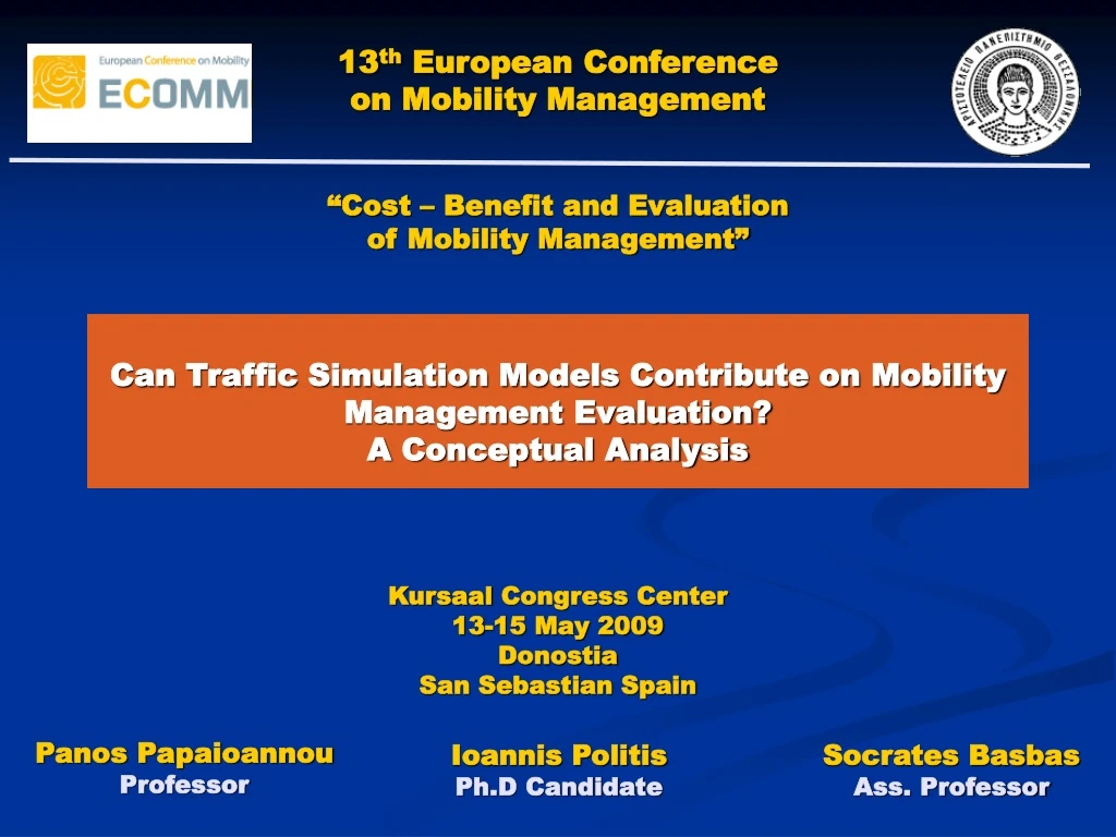
13th European Conference on Mobility Management “Cost – Benefit and Evaluation of Mobility Management” Can Traffic Simulation Models Contribute on Mobility Management Evaluation? A Conceptual Analysis Kursaal Congress Center 13-15 May 2009 Donostia San Sebastian Spain Panos Papaioannou Professor Ioannis Politis Ph.D Candidate Socrates Basbas Ass. Professor
PRESENTATION OUTLINE • Objectives and Applications of Transport Planning Tools • Transportation Models and Benchmarking Evaluation • Introducing TPT into Mobility Management Evaluation • Conclusions and Discussion • Annex: Case Study – Classical Approach
KEY QUESTION Why it is Important to Use Transportation Planning Software Tools ??
REASONS • Transportation System: Complex multi-dimensional factors • not easily determined, measured or estimated directly • Impact Estimations (ex ante!) derived from • the construction of a new road infrastructure • or operation of a new transport mode, • or….implementation of a MM plan! • Impact Estimations: • - The transportation system itself • - The environmental effects and the potential revenues • - The redistribution of the land use • Easier to Introduce Transport Planning Theories
OBJECTIVE OF TRANSPORT PLANNING & SIMULATION TOOL • To represent with accuracy the underlying operation of • the transport system • (in terms of traffic conditions and travel patterns) • To create reliable mathematical models for testing • different / various schemes at the base year (underlying) • or at future years (planning horizons ) • These schemes pertain to be at the supply (new • infrastructure, new mode, pedestrialization of roads etc) • or the demand (car pooling, flexible working hours etc) • side
OBJECTIVE OF TRANSPORT PLANNING & SIMULATION TOOL • A simulation traffic model can estimate the impacts derived from a Mobility Management Measure, primarily on the demand changes. • In fact, a MMM (such as car pooling, van pooling, flexible or staggered working hours etc.) is translated into changes at the Origin – Destination Matrices of each respective demand segment and changes in travel chain in general. • An evident disadvantage is that existing simulation tools just “simulate” the anticipated improvements of a network. The reality proves that when the traffic conditions are improved new (generated) traffic is added (the vicious circle of the transportation systems)
TRAVEL PATTERNS EXAMPLE Production trips Attraction Trips
APPLICATIONS OF TRANSPORT PLANNING SOFTWARE TOOLS • Traffic and Transportation Studies • Feasibility (Socio – Economic) Studies • Cost – Benefit Studies • Urban Planning Studies • Environmental Studies • Mode Choice and Travel Behavior Studies!!
Transportation Models and Benchmarking Evaluation • According to the HCM (2000) a transportation model is: • “A computer program that uses mathematical models to conduct experiments with traffic events on a transportation facility or system over extended periods of time” • Transportation Models Classification: • * According to their application area • * According to the level of presentation of the traffic flows • * According to the time period of the analysis
Transportation Models Classification
Macroscopic Models • Take into account transportation network attributes • such as capacity, speed limit, flow and density • Simulate large scale facilities (highways, regions etc) • No need to track individual vehicles (aggregate theory) • No detailed information about road design and signal • plans is needed • CUBE, TRIPS and VISUM
Mesoscopic Models • Take into account the actual road geometry and signal • timing plans • Simulate intersections in a corridor or city • Simulate individual vehicles • Describe activities based on aggregate or macroscopic • level • SATURN, CORSIM, TRANSCAD, EMME/3, AIMSUN
Microscopic Models • Simulate characteristics and interactions of individual • vehicles • Study area: Intersection or a road segment • (e.g. a corridor ) • Enclose theories and rules for vehicle acceleration, • passing manoeuvres and lane-changing • PARAMICS, VISSIM, AIMSUN
Comparative Analysis of the most commonly used transportation software
Existed Transport and Simulation Models The analysis is based only on Quantitative Data/Results !!
KEY QUESTIONS • What are the user needs of the study area? • How much dependent the users are to their cars? • What will be the overall impacts of a “real” Mobility • Management Measure (MMM) to the Study area • Which MMM is the most promising to this specific area • Which are the potential barriers to implement them? • The Qualitative or Quantitative data should be taken into • consideration most? The same?
A Conceptual Framework of Introducing Transportation Models into Mobility Management Measures Evaluation and Classification
Planning Phase • The MMM that will be examined should be linked with the • trip purposes of the study area (different demand matrices) • Why not to follow the categorization of MMM derived from • MAX project? • A well structured questionnaire should • Estimate the behavioral stage of the targeted • population (why not the diagnostic questions?) • Identify the user needs (that wanted or expected) and • the level of acceptance of the examined MMM through • well known–used techniques
Planning Phase • The criteria of evaluation should be clearly determined • Transportation indices (VKT, Speed, Delays etc.) • Environmental indices (CO, HC, NOx etc.) • Level of maturity (Low, Medium, High) • Change on Behavioral Stage (0 stage, 1 stage, …3 stages) • The selection of the appropriate Transportation Model • should be based on: • The criteria of evaluation • The area under consideration (macro,meso,micro)
Analysis Phase • The criteria and sub-criteria (quantitative and qualitative) • should get an evaluation grade • All the criteria should also obtain weights (experts survey) • Well know multi criteria decision analysis tools (MCDA) • could easily apply the weights to the grades • ( software : HIPRE 3+, web-HIPRE, EXPERT Choice model)
Classification Phase • The evaluation grade for the qualitative criteria are based • on subjective judgment • Various techniques can quantify the qualitative criteria • ( e.g. Evidentional Reasoning Approach) • If the initial evaluation criteria are properly selected, then • the final ranking of the MMM will include qualitative • parameters such as the trip purpose, the behavioral stage • etc. which are not included in conventional evaluations • Alternatively, the proposed methods could be classified • through a cost benefit analysis (all the benefits are • translated into momentary units – classical approach)
CONCLUSIONS • Mobility Management seems to be adopted more and more by local authorities • It is important to have accurate estimations about the most promising MMM “before moving out of the office” • The classical transportation planning theory cannot include qualitative parameters especially from the behavioural – psychology side
CONCLUSIONS • These parameters are equal important since can affect the effectiveness of a measure • A new framework should be established combining the knowledge obtained from transportation planning theories and psychology behavioural science
Thank you for your attention!! Ioannis K. Politis ------------------------------------- Ph.D. Candidate Laboratory of Transportation and Construction Management Department of Civil Engineering Aristotle University of Thessaloniki, Greece pol@civil.auth.gr
ANNEX Case Study The use of a mesoscopic traffic analysis model in order to run alternative road charging schemes at the Outer Ring Road of Thessaloniki
THE STUDY HIGHWAY • 35 km length freeway • Estimated budget of 700 million euros • Will offer connections to the Inner Ring Road • 13 Bridges with a total length of 2 km • 20 Tunnels with a total length of 20 km • 9 Interchanges • Completion date: 2016
THE EVALUATION MODEL • Mesoscopic Model SATURN (Simulation and • Assignment of Traffic to Urban Road Networks) • Extended network was coded (base year 2006): • *783 simulation nodes including: • 27 external nodes • 310 priority junctions • 292 traffic signals • 154 dummy nodes • *2508 simulation links • *6350 simulation turns • *210 traffic zones • Morning Peak Period 08:00-09:00 • Ap. 200 traffic counts were used for calibration purposes • (180 for new O-D matrix estimation and 20 for validation)
THE EVALUATION MODEL Modeled vs Observed Flows
DETAILED REPRESENTATION OF THE INTERSECTIONS IC # 1-2 : Interchange to the Inner Ring Road
DETAILED REPRESENTATION OF THE INTERSECTIONS IC # 6 : Panorama
Flat_Tolls Marginal Revenue Curve Distance_Based_Tolls 25000 Poly. (Flat_Tolls) Poly. (Distance_Based_Tolls) 23000 2 y = -0,0002x + 4,4287x + 40 21000 19000 17000 15000 Total Hourly Revenues (in euros) 13000 2 y = -3E-06x + 0,5497x + 40 11000 9000 7000 5000 10000 12000 14000 16000 18000 20000 22000 Total Flows (Quantity) NUMERICAL RESULTS
KEY FINDINGS OF THE STUDY • The distance based tolls frustrate journeys > 20 km • The average journey length varies between 12-15 km for • all the methods and toll rate levels examined • The demand is inelastic (- 1 < e < 0) for all the examined • scenarios, especially for the East – West Direction • Flat tolls schemes lead into more elastic interrelations • with respect to demand (actual flow)
KEY FINDINGS OF THE STUDY OBTAINED REVENUES • Flat Tolls : The optimum toll value should be greater than • 2 euros • Higher toll level will lead to lower actual flows • and accordingly to bigger obtained revenues • Distance Based Tolls: The optimum toll value should be • lower than 0.087 euros/km • Lower toll level will lead to higher • actual flows and accordingly to • bigger obtained revenues