Download
1 / 36
360 likes | 554 Vues
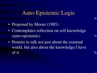
Auto-Epistemic Logic. Proposed by Moore (1985) Contemplates reflection on self knowledge (auto-epistemic) Allows for representing knowledge not just about the external world, but also about the knowledge I have of it. Syntax of AEL.

E N D
Auto-Epistemic Logic • Proposed by Moore (1985) • Contemplates reflection on self knowledge (auto-epistemic) • Allows for representing knowledge not just about the external world, but also about the knowledge I have of it
Syntax of AEL • 1st Order Logic, plus the operator L (applied to formulas) • Lj means “I know j” • Examples: MScOnSW →L MScOnSW (or L MScOnSW → MScOnSW) young (X) Lstudies (X) → studies (X)
Meaning of AEL • What do I know? • What I can derive (in all models) • And what do I not know? • What I cannot derive • But what can be derived depends on what I know • Add knowledge, then test
Semantics of AEL • T* is an expansion of theory T iff T* = Th(T{Lj : T* |= j} {Lj : T* |≠j}) • Assuming the inference rule j/Lj : T* = CnAEL(T {Lj : T* |≠j}) • An AEL theory is always two-valued in L, that is, for every expansion: j | Lj T* Lj T*
Knowledge vs. Belief • Belief is a weaker concept • For every formula, I know it or know it not • There may be formulas I do not believe in, neither their contrary • The Auto-Epistemic Logic of knowledge and Belief (AELB), introduces also operator B j – I believe in j
AELB Example • I rent a film if I believe I’m neither going to baseball nor football games Bbaseball Bfootball → rent_filme • I don’t buy tickets if I don’t know I’m going to baseball nor know I’m going to football Lbaseball Lfootball → buy_tickets • I’m going to football or baseball baseball football • I should not conclude that I rent a film, but do conclude I should not buy tickets
Axioms about beliefs • Consistency Axiom B • Normality Axiom B(F → G) → (B F →B G) • Necessitation rule F B F
Some consequences of the Axioms • B(F /\ G) ≡B F /\B G • BF → BF • B(F \/ G) →BF \/BG
Minimal models • In what do I believe? • In that which belongs to all preferred models • Which are the preferred models? • Those that, for one same set of beliefs, have a minimal number of true things • A model M is minimal iff there does not exist a smaller model N, coincident with M on Bj e Lj atoms • When j is true in all minimal models of T, we write T |=minj
AELB expansions • T* is a static (autoepistemic) expansion of T iff T* = CnAELB(T {Lj : T* |≠j} {Bj : T* |=minj}) where CnAELB denotes closure using the axioms of AELB plus necessitation for L
Some properties of static autoepistemic expansions • T* |= Lj iff T* |= j • T* |= Bjif T* |=minj • The other direction of the last implication only holds for particular cases (e.g. rational theories – those without positive occurrences of belief atoms).
The special case of AEB • Because of its properties, the case of theories without the knowledge operator is especially interesting • The definition of expansion becomes: T* = YT(T*) where YT(T*) = CnAEB(T {Bj : T* |=minj}) and CnAEB denotes closure using the axioms of AEB
Least expansion • Theorem: Operator Y is monotonic, i.e. T T1 T2→YT(T1) YT(T2) • Hence, there always exists a minimal expansion of T, obtainable by transfinite induction: • T0 = CnAEB(T) • Ti+1 = YT(Ti) • Tb = Ua < b Ta (for limit ordinals b)
Consequences • Every AEB theory has at least one expansion • If a theory is affirmative (i.e. all clauses have at least a positive literal) then it has at least a consistent expansion • There is a procedure to compute the semantics
Example • BEarthquake /\ BFires Calm • B(Earthquake \/ Fires) Worried • BEarthquake /\ BFires Panicked • BCalm CallHome • Earthquake \/ Fires
Computation of Static Completion • T0 = CnAEB(T) • T0 |= Earthquake \/ Fires • T0 |=minEarthquake \/ Fires • T1 = YT(T0)= CnAEB(T0 {Bj : T0 |=minj}) • T1 = CnAEB(T0 {B(Eq \/ Fi), B(Eq \/ Fi),…}) • T1 |= Worried • T1 |= BEarthquake \/ BFires • T1 |= B Earthquake \/ B Fires • T1 |=minCalm and T1 |=minPanicked
Static Completion (cont.) • T2 = YT(T1)= CnAEB(T1 {Bj : T1 |=minj}) • T2 = CnAEB(T1 {B(Eq \/ Fi), B(Eq \/ Fi), BCalm, BPanicked, BWorried,… }) • T2 |= CallHome • T3 = YT(T2)= CnAEB(T2 {Bj : T2 |=minj}) • T2 = CnAEB(T1 {B(Eq \/ Fi), B(Eq \/ Fi), BCalm, BPanicked, BWorried, BCallHome, … })
LP forKnowledge Representation • Due to its declarative nature, LP has become a prime candidate for Knowledge Representation and Reasoning • This has been more noticeable since its relations to other NMR formalisms were established • For this usage of LP, a precise declarative semantics was in order
Language • A Normal Logic Programs P is a set of rules: H ¬A1, …, An, not B1, … not Bm (n,m ³ 0) where H, Ai and Bj are atoms • Literal not Bj are called default literals • When no rule in P has default literal, P is called definite • The Herbrand base HP is the set of all instantiated atoms from program P. • We will consider programs as possibly infinite sets of instantiated rules.
Declarative Programming • A logic program can be an executable specification of a problem member(X,[X|Y]). member(X,[Y|L])¬ member(X,L). • Easier to program, compact code • Adequate for building prototypes • Given efficient implementations, why not use it to “program” directly?
flight from to flight ( lisbon , adam ). Lisbon Adam Þ flight ( lisbon , london ) Lisbon London M M M ¬ connection ( A , B ) flight ( A , B ). ¬ connection ( A , B ) flight ( A , C ), connection ( C , B ). ¬ chooseAnot her ( A , B ) not connection ( A , B ). LP and Deductive Databases • In a database, tables are viewed as sets of facts: • Other relations are represented with rules:
¬ connection ( A , B ) flight ( A , B ). ¬ connection ( A , B ) flight ( A , C ), connection ( C , B ). ¬ chooseAnot her ( A , B ) not connection ( A , B ). LP and Deductive DBs (cont) • LP allows to store, besides relations, rules for deducing other relations • Note that default negation cannot be classical negation in: • A form of Closed World Assumption (CWA) is needed for inferring non-availability of connections
¬ flies ( A ) bird ( A ), not abnormal ( A ) . ¬ bird ( P ) penguin ( P ). ¬ abnormal ( P ) penguin ( P ). bird ( a ). penguin ( p ). Default Rules • The representation of default rules, such as “All birds fly” can be done via the non-monotonic operator not
The need for a semantics • In all the previous examples, classical logic is not an appropriate semantics • In the 1st, it does not derive not member(3,[1,2]) • In the 2nd, it never concludes choosing another company • In the 3rd, all abnormalities must be expressed • The precise definition of a declarative semantics for LPs is recognized as an important issue for its use in KRR.
2-valued Interpretations • A 2-valued interpretation I of P is a subset of HP • A is true in I (ie. I(A) = 1) iff AÎ I • Otherwise, A is false in I (ie. I(A) = 0) • Interpretations can be viewed as representing possible states of knowledge. • If knowledge is incomplete, there might be in some states atoms that are neither true nor false
3-valued Interpretations • A 3-valued interpretation I of P is a set I = T U not F where T and F are disjoint subsets of HP • A is true in I iff A Î T • A is false in I iff AÎ F • Otherwise, A is undefined (I(A) = 1/2) • 2-valued interpretations are a special case, where: HP = T U F
Lattice-valued interpretations • We can generalize the previous definition to an arbitrary lattice of truth-values • Let L be a complete lattice then an interpretation of a program P is a mapping I:HP→ L • Notice that any complete lattice has a least element () and a top element (T) , so a “true” proposition is mapped into T while a “false” proposition is mapped into . • Some interesting useful complete lattices: • {0,1} with 0 < 1. • {0,1/2,1} with 0 < 1/2 < 1 • [0,1] • Belnap’s four valued logic with with 0 <unknown | contradictory < 1
Intermezzo: lattices • A partially ordered set (poset) is a set equipped with a reflexive, antisymmetric and transitive binary relation ≤: • Reflexivity: a ≤ a • Antisymmetry: if a ≤ b and b ≤ a then a=b • Transitivity: if a ≤ b and b ≤ c then a ≤ c • A lattice is a poset such that for any two elements x and y the set {x,y} has both a least upper bound (join or supremum - \/) and a greatest lower bound (meet or infimum - /\). The join and meet obey to the following properties: • Commutative laws: a \/ b = b \/ a, and a /\ b = b /\ a • Associative laws: a \/ (b \/ c)= (a \/ b) \/ c, and a /\ (b /\ c)= (a /\ b) /\ c • Absorption laws: a \/ (a /\ b)= a, and a /\ (a \/ b)= a • Notice that x ≤ y iff x = x /\ y, or equivalently y = x \/ y. • A complete lattice is a lattice where all subsets have a join and a meet.
Models • Models can be defined via an evaluation function Î: • For an atom A, Î(A) = I(A) • For a formula F, Î(not F) = T - Î(F) (for lattices with complement) • For formulas F and G: • Î((F,G)) = glb(Î(F), Î(G)) • Î((F;G)) = lub(Î(F), Î(G)) • Î(F ¬ G)= T iff Î(F) ≥ Î(G). • I is a model of P iff, for all rule H ¬ B of P: Î(H ¬ B) = T
¬ ableMathem atician ( X ) physicist ( X ) physicist ( einstein ) president ( cavaco ) Minimal Models Semantics • The idea of this semantics is to minimize positive information. What is implied as true by the program is true; everything else is false. • {pr(c),pr(e),ph(s),ph(e),aM(c),aM(e)} is a model • Lack of information that cavaco is a physicist, should indicate that he isn’t • The minimal model is: {pr(c),ph(e),aM(e)}
Minimal Models Semantics • [Truth ordering] For interpretations I and J, I £ J iff for all atom A, I(A) £ I(J), i.e. for the case of 2-valued interpretations TIÍ TJ and FIÊ FJ • Every definite logic program has a least (truth ordering) model. • [minimal models semantics] An atom A is true in (definite) P iff A belongs to its least model. Otherwise, A is false in P.
TP operator (2-valued case) • The minimal models of a definite P can be computed (bottom-up) via operator TP • [TP] Let I be an interpretation of definite P. TP(I) = {H: (H ¬ Body) Î P and Body Í I} • If P is definite, TP is monotone and continuous. Its minimal fixpoint can be built by: • I0 = {} and In = TP(In-1) with n > 0 • The least model of definite P is TPw({})
TP operator (L-valued case) • [TP] Let I be an interpretation of definite P. TP(I)(H) = lub{Î(Body): (H ¬ Body) Î P} • If P is definite, TP is monotone. Its minimal fixpoint can be built by iterating the TP operator: • I0 = TP0={} • Iα = TP α = TP(Iα -1) = TP (TP α-1), where α is a successor ordinal • Iβ = TP b = |_| α < βTP α = |_| α < β Iα where βis a limit ordinal
TP operator (L-valued case) • There is a successor ordinal lsuch that TP l = TP l-1 , i.e. there is a least fixpoint of TP. Furthermore, the least model of definite program P coincides with the least fixpoint of TP.In general, more than w iterations might be needed to reach the least fixpoint. However, if lattice L is finite then at most w iterations are enough.
Computation of minimal models • For the 2-valued case there is a complete method: SLD resolution (Linear resolution with a selection function for definite sentences). • A SLD-goal of the form← A1, …, Am, L, C1, …, Cnhas a successor ← (A1, …, Am, B1, …, Bk, C1, …, Cn ) θfor each rule H :- B1, …, Bk, belonging to the program such that L and H unify with mgu θ. • A SLD-derivation is a sequence of applications of SLD-resolution, and a SLD-refutation is a SLD-derivation which ends in the empty clause, i.e. no goals after ←. • For the lattice-valued case, there are proof procedures based on tabulation methods, which we will not present.
On Minimal Models • SLD can be used as a proof procedure for the minimal models semantics: • If the is a SLD-derivation for A, then A is true • Otherwise, A is false • The semantics does not apply to normal programs: • p ¬ not q has two minimal models: {p} and {q} There is no least model !