Comprehensive Drawing Algorithms for Lines, Curves, and Circles
Learn efficient line drawing, Bresenham's algorithm, circle drawing techniques, and OpenGL programming for 2D graphics.

Comprehensive Drawing Algorithms for Lines, Curves, and Circles
E N D
Presentation Transcript
UNIT- I 2D PRIMITIVES
Line Drawing y = m . x + b m = (yend – y0) / (xend – x0) b = y0 – m . x0 yend y0 x0 xend
DDA Algorithm if |m|<1 xk+1 = xk + 1 yk+1 = yk + m if |m|>1 yk+1 = yk + 1 xk+1 = xk + 1/m yend y0 x0 xend yend y0 xend x0
DDA Algorithm #include <stdlib.h> #include <math.h> inline int round (const float a) { return int (a + 0.5); } void lineDDA (int x0, int y0, int xEnd, int yEnd) { int dx = xEnd - x0, dy = yEnd - y0, steps, k; float xIncrement, yIncrement, x = x0, y = y0; if (fabs (dx) > fabs (dy)) steps = fabs (dx); /* |m|<1 */ else steps = fabs (dy); /* |m|>=1 */ xIncrement = float (dx) / float (steps); yIncrement = float (dy) / float (steps); setPixel (round (x), round (y)); for (k = 0; k < steps; k++) { x += xIncrement; y += yIncrement; setPixel (round (x), round (y)); } }
Bresenham’s Line Algorithm yk+1 yk xk xk+1 yk+1 du y dl yk xk xk+1
Bresenham’s Line Algorithm #include <stdlib.h> #include <math.h> /* Bresenham line-drawing procedure for |m|<1.0 */ void lineBres (int x0, int y0, int xEnd, int yEnd) { int dx = fabs(xEnd - x0), dy = fabs(yEnd - y0); int p = 2 * dy - dx; int twoDy = 2 * dy, twoDyMinusDx = 2 * (dy - dx); int x, y; /* Determine which endpoint to use as start position. */ if (x0 > xEnd) { x = xEnd; y = yEnd; xEnd = x0; } else { x = x0; y = y0; } setPixel (x, y); while (x < xEnd) { x++; if (p < 0) p += twoDy; else { y++; p += twoDyMinusDx; } setPixel (x, y); } }
Circle Drawing Pythagorean Theorem: x2 + y2 = r2 (x-xc)2 + (y-yc)2 = r2 (xc-r) ≤ x ≤ (xc+r) y = yc± √r2 - (x-xc)2 (x, y) r yc xc
Circle Drawing change x change y
Circle Drawing using polar coordinates x = xc + r . cos θ y = yc + r . sin θ change θ with step size 1/r (x, y) r θ (xc, yc)
Circle Drawing using polar coordinates x = xc + r . cos θ y = yc + r . sin θ change θ with step size 1/r use symmetry if θ>450 (x, y) r θ (xc, yc) (y, -x) (y, x) (-x, y) (x, y) 450 (xc, yc)
Midpoint Circle Algorithm f(x,y) = x2 + y2 - r2 <0 if (x,y) is inside circle f(x,y) =0 if (x,y) is on the circle <0 if (x,y) is outside circle use symmetry if x>y yk yk-1/2 yk-1 xk xk+1
Midpoint Circle Algorithm /* Calculate next points and plot in each octant. */ while (circPt.x < circPt.y) { circPt.x++; if (p < 0) p += 2 * circPt.x + 1; else { circPt.y--; p += 2 * (circPt.x - circPt.y) + 1; } circlePlotPoints (circCtr, circPt); } } void circlePlotPoints (scrPt circCtr, scrPt circPt); { setPixel (circCtr.x + circPt.x, circCtr.y + circPt.y); setPixel (circCtr.x - circPt.x, circCtr.y + circPt.y); setPixel (circCtr.x + circPt.x, circCtr.y - circPt.y); setPixel (circCtr.x - circPt.x, circCtr.y - circPt.y); setPixel (circCtr.x + circPt.y, circCtr.y + circPt.x); setPixel (circCtr.x - circPt.y, circCtr.y + circPt.x); setPixel (circCtr.x + circPt.y, circCtr.y - circPt.x); setPixel (circCtr.x - circPt.y, circCtr.y - circPt.x); } #include <GL/glut.h> class scrPt { public: GLint x, y; }; void setPixel (GLint x, GLint y) { glBegin (GL_POINTS); glVertex2i (x, y); glEnd ( ); } void circleMidpoint (scrPt circCtr, GLint radius) { scrPt circPt; GLint p = 1 - radius; circPt.x = 0; circPt.y = radius; void circlePlotPoints (scrPt, scrPt); /* Plot the initial point in each circle quadrant. */ circlePlotPoints (circCtr, circPt);
OpenGL #include <GL/glut.h> // (or others, depending on the system in use) void init (void) { glClearColor (1.0, 1.0, 1.0, 0.0); // Set display-window color to white. glMatrixMode (GL_PROJECTION); // Set projection parameters. gluOrtho2D (0.0, 200.0, 0.0, 150.0); } void lineSegment (void) { glClear (GL_COLOR_BUFFER_BIT); // Clear display window. glColor3f (0.0, 0.0, 1.0); // Set line segment color to red. glBegin (GL_LINES); glVertex2i (180, 15); // Specify line-segment geometry. glVertex2i (10, 145); glEnd ( ); glFlush ( ); // Process all OpenGL routines as quickly as possible. } void main (int argc, char** argv) { glutInit (&argc, argv); // Initialize GLUT. glutInitDisplayMode (GLUT_SINGLE | GLUT_RGB); // Set display mode. glutInitWindowPosition (50, 100); // Set top-left display-window position. glutInitWindowSize (400, 300); // Set display-window width and height. glutCreateWindow ("An Example OpenGL Program"); // Create display window. init ( ); // Execute initialization procedure. glutDisplayFunc (lineSegment); // Send graphics to display window. glutMainLoop ( ); // Display everything and wait. }
OpenGL Point Functions • glVertex*( ); * : 2, 3, 4 i (integer) s (short) f (float) d (double) Ex: glBegin(GL_POINTS); glVertex2i(50, 100); glEnd(); int p1[ ]={50, 100}; glBegin(GL_POINTS); glVertex2iv(p1); glEnd();
OpenGL Line Functions • GL_LINES • GL_LINE_STRIP • GL_LINE_LOOP Ex: glBegin(GL_LINES); glVertex2iv(p1); glVertex2iv(p2); glEnd();
OpenGL glBegin(GL_LINES); GL_LINES GL_LINE_STRIP glVertex2iv(p1); glVertex2iv(p2); glVertex2iv(p3); glVertex2iv(p4); glVertex2iv(p5); glEnd(); GL_LINE_LOOP p3 p3 p5 p1 p1 p2 p4 p2 p4 p3 p5 p1 p2 p4
Antialiasing Supersampling Count the number of subpixels that overlap the line path. Set the intensity proportional to this count.
Antialiasing Area Sampling Line is treated as a rectangle. Calculate the overlap areas for pixels. Set intensity proportional to the overlap areas. 80% 25%
Antialiasing Pixel Sampling Micropositioning Electron beam is shifted 1/2, 1/4, 3/4 of a pixel diameter.
Line Intensity differences Change the line drawing algorithm: • For horizontal and vertical lines use the lowest intensity • For 45o lines use the highest intensity
Matrices • A matrix is a rectangular array of numbers. • A general matrix will be represented by an upper-case italicised letter. • The element on the ith row and jth column is denoted by ai,j. Note that we start indexing at 1, whereas C indexes arrays from 0.
Matrices – Addition • Given two matrices A and B if we want to add B to A (that is form A+B) then if A is (nm), B must be (nm), Otherwise, A+B is not defined. • The addition produces a result, C = A+B, with elements:
Matrices – Multiplication • Given two matrices A and B if we want to multiply B by A (that is form AB) then if A is (nm), B must be (mp), i.e., the number of columns in A must be equal to the number of rows in B. Otherwise, AB is not defined. • The multiplication produces a result, C = AB, with elements: (Basically we multiply the first row of A with the first column of B and put this in the c1,1 element of C. And so on…).
Matrices – Multiplication (Examples) 26+ 63+ 72=44 Undefined! 2x2 x 3x2 2!=3 2x2 x 2x4 x 4x4 is allowed. Result is 2x4 matrix
Matrices -- Basics • Unlike scalar multiplication, AB ≠ BA • Matrix multiplication distributes over addition: A(B+C) = AB + AC • Identity matrix for multiplication is defined as I. • The transpose of a matrix, A, is either denoted ATor A’ is obtained by swapping the rows and columns of A:
Translate Shear Rotate Scale 2D Geometrical Transformations
P’(x’,y’) dy P(x,y) dx Translate Points Recall.. We can translate points in the (x, y) plane to new positions by adding translation amounts to the coordinates of the points. For each point P(x, y) to be moved by dx units parallel to the x axis and by dy units parallel to the y axis, to the new point P’(x’, y’ ). The translation has the following form: In matrix format: If we define the translation matrix , then we have P’ =P + T.
P(x,y) y sy y P’(x’,y’) sx x x Scale Points • Points can be scaled (stretched) by sx along the x axis and by sy along the y axis into the new points by the multiplications: • We can specify how much bigger or smaller by means of a “scale factor” • To double the size of an object we use a scale factor of 2, to half the size of an obejct we use a scale factor of 0.5 If we define , then we have P’ =SP
P’(x’,y’) P(x,y) y l y’ O x’ x Rotate Points (cont.) Points can be rotated through an angle about the origin: P’ =RP
Review… • Translate: P’ = P+T • Scale: P’ = SP • Rotate: P’ = RP • Spot the odd one out… • Multiplying versus adding matrix… • Ideally, all transformations would be the same.. • easier to code • Solution: Homogeneous Coordinates
Homogeneous Coordinates For a given 2D coordinates (x, y), we introduce a third dimension: [x, y, 1] In general, a homogeneous coordinates for a 2D point has the form: [x, y, W] Two homogeneous coordinates [x, y, W] and [x’, y’, W’] are said to be of the same (or equivalent) if x = kx’ eg: [2, 3, 6] = [4, 6, 12] y = ky’ for some k≠ 0 where k=2 W = kW’ Therefore any [x, y, W] can be normalised by dividing each element by W: [x/W, y/W, 1]
Homogeneous Transformations Now, redefine the translation by using homogeneous coordinates: Similarly, we have: Scaling Rotation P’ = S P P’ = R P
Composition of 2D Transformations • Additivity of successive translations • We want to translate a point P to P’ by T(dx1, dy1) and then to P’’ by another T(dx2, dy2) • On the other hand, we can define T21= T(dx1, dy1) T(dx2, dy2) first, then apply T21 to P: • where
(1,3) T(-1,2) T(1,-1) (2,2) (2,1) Examples of Composite 2D Transformations
Composition of 2D Transformations (cont.) • Multiplicativity of successive scalings • where
Composition of 2D Transformations (cont.) • 3. Additivity of successive rotations • where
Composition of 2D Transformations (cont.) • 4. Different types of elementary transformations discussed above can be concatenated as well. • where
Consider the following two questions: • translate a line segment P1 P2, say, by -1 units in the x direction and -2 units in the y direction. • 2). Rotate a line segment P1 P2, say by degrees counter clockwise, about P1. P2(3,3) P’2 P1(1,2) P’1 P’2 P2(3,3) P’1 P1(1,2)
P2 P2(3,3) P2 T(-1,-2) R() T(1,2) P1 P2(2,1) P1(1,2) P1 P1 Other Than Point Transformations… Translate Lines: translate both endpoints, then join them. Scale or Rotate Lines: More complex. For example, consider to rotate an arbitrary line about a point P1, three steps are needed: 1). Translate such that P1 is at the origin; 2). Rotate; 3). Translate such that the point at the origin returns to P1.
Another Example. Translate Translate Rotate Scale
Order Matters! As we said, the order for composition of 2D geometrical transformations matters, because, in general, matrix multiplication is not commutative. However, it is easy to show that, in the following four cases, commutativity holds: 1). Translation + Translation 2). Scaling + Scaling 3). Rotation + Rotation 4). Scaling (with sx = sy) + Rotation just to verify case 4: if sx = sy, M1 = M2.
Rigid-Body vs. Affine Transformations A transformation matrix of the form where the upper 22 sub-matrix is orthogonal, preserves angles and lengths. Such transforms are called rigid-body transformations, because the body or object being transformed is not distorted in any way. An arbitrary sequence of rotation and translation matrices creates a matrix of this form. The product of an arbitrary sequence of rotation, translations, and scale matrices will cause an affine transformation, which have the property of preserving parallelism of lines, but not of lengths and angles.
Rigid- body Transformation Affine Transformation 45º Unit cube Scale in x, not in y Shear in the x direction Shear in the y direction Rigid-Body vs. Affine Transformations (cont.) Shear transformation is also affine.
2D Output Primitives Points Lines Circles Ellipses Other curves Filling areas Text Patterns Polymarkers
Filling area Polygons are considered! Scan-Line Filling (between edges) Interactive Filling (using an interior starting point)
1) Scan-Line Filling (scan conversion) Problem: Given the vertices or edges of a polygon, which are the pixels to be included in the area filling?
Scan-Line filling, cont’d Main idea: locate the intersections between the scan-lines and the edges of the polygon sort the intersection points on each scan-line on increasing x-coordinates generate frame-buffer positions along the current scan-line between pairwise intersection points