Download
1 / 39
390 likes | 566 Vues
Applications Engineer Approach to Maxwell and Other Mathematically Intense Problems. Or Applications Engineers Don’t Do Hairy Math. Marcus O Durham, PhD, PE Fellow, IEEE Theway Corp. Robert A Durham, PE Member, IEEE D 2 Tech Solutions, Inc. Karen D Durham, EI Member, NSPE NATCO.

E N D
Applications Engineer Approach to Maxwell and Other Mathematically Intense Problems Or Applications Engineers Don’t Do Hairy Math Marcus O Durham, PhD, PEFellow, IEEE Theway Corp Robert A Durham, PE Member, IEEE D2 Tech Solutions, Inc. Karen D Durham, EI Member, NSPE NATCO
Objective • Develop a structure for app engineers to use when reading or working with complex math concepts
Abstract • EE taught w/ complex concepts and intense math • In practice, very little intricate science • Problems solved with algebra • Why is there a difference? • Paper reduces all EE math totwo simple equations
Abstract too • Single Unified Equation (SUE) for circuits • Add distance to encompass Maxwell’s suite • Math is vector algebra • NO CALCULUS
But First… • Would you agree that apps engineers… • Are results oriented? • Solve problems w/out complex theory? • Don’t even read articles w/ hairy math? • Can’t remember Maxwell? • Think a curl is part of the Winter Olympics? • Then this article is for you.
Core Belief • Kirchhoff is used to solve all problems • Kirchhoff derived from Maxwell • Ergo - Maxwell is at the core of all EE • However, how many EEs can do derivation w/out reference? • And how many EE books can be used for reference?
MATH Core Belief • We’re not messing with Kirchhoff • We are cleaning up Maxwell • We are eliminating Calculus • And Diff-EQ and Partials • And others that App Engineers don’t use • Allows comprehension of intense articles w/out following the hairy math
Are we together so far? Okay then . . .
P’s and Q’s • Three elements of matter • Mass (m) • Magnetic Pole (p or φ) • Charge (q)Equations use elementalrather than derived
Time is on Our Side • Time is always a denominator • Three elements of time • Fixed: t = 1 • Rate: 1/tt~ Velocity (Current), Energy • Acceleration: 1/(tt tr) ~ Potential, Power
To the Point • Electrical and magnetic concepts can be combined into one simple equation.i.e. • Electromagnetic energy is the change in the product of charge and pole strength over time
E = [p q] / tt • Equation is for point conditions (node) • Concept so fundamental and inclusive appears intuitively obvious • However, NO previous references
What are Measurables? • Can only measure three things • Voltage : V = [p]/t • Current : I = [q]/t • Frequency: f = 1 /t • All measurables derived from SUE • That’s a strong statement!
Calculating… • Can only calculate three things • Measured components are unique, so can’t add or subtract • Leaves multiplication and division
Calculating… • Product S = V*I = [p/tr] * [q/tt] = [E]/tr • Ratio Z = V/I= [p/tr] / [q/tt] • Delay or phase shift td = tr – tt • Anything else?
Are the Laws Legal? • Concepts embedded in SUE are staggering • KVL • KCL • Faraday • Definitions of “Measurables” • At a node, this is all encompassing • No more complex than algebra
E = [p q] / tt • This opens the understanding of electromagnetic science to an entire new level of application. • The equation removes the constraints on moving between electrics and magnetics • “But what about Fields?”
Fields are a Gas • E-mag fields considered “toughest” part of EE • Actually, no more complex than circuits • As a circuit is analogous to liquid flow… • Fields are analogous to gas in a vessel!
Space, the Final Frontier • Cartesian axes good for straight, rectangular world • Real world is curvilinear, spheroidal space • Fields live on the surface of a spheroid • A coordinate system based on a sphere is necessary
y x t s Spherical Coordinates • Corresponds to navigation coordinates t ~ latitude s ~ longitude y ~ altitude
z dt bs bys θ y sy x st ss Spherical Coordinates • bys defines a point on the surface relative to the origin • dt defines the distance aroundthe sphere for a given “parallel”
Moving and Mooning • Consider the sphere to be a moon orbiting around a “fixed” planet • How does the moon move? • Rotational (days) • Orbital (months) • The combination creates sinusoidal motion
Or • Consider the magnetic rotation of a motor • How does the motor work? • Rotational (shaft) • Orbital (coils) • The combination creates sinusoidal motion
Crank out the Volume • Surface volume • Calculated from longitude, latitude and altitude • Uses vector algebra • Vy= ss st sy • Operational volume • Region transcribed by motion of the sphere (under sinusoid in 3D) • Vy = bys dt sy • Space vector (sy) describesthe orbital motion
If you build it… So, what’s the deal withspheres and volumes?
Here’s the pitch • The Simplified Unified Equation • Multiplied by the ratio of • Operational Volume to Surface Volume • Yields electromagnetic field energy
Going, Going • What is the significance of this simple product of flux, charge and distances over time?
And it’s Outta Here • Every machines, transmission and fields problem calculated from one simple relationship • Complex, special problems solved using simple program or spreadsheet
Density • Current not point but dispersed • Skin Effect • Circumference determines cross-sectional area (At) • Current Density (Jt) = current over area • Charge Density (ρ) = charge over volume
Intensity of the Density • Field Intensity 1 / (time * length) • Field Density 1 / Area • Energy is the product of intensity, density and volume • All four foundational relationships can be derived from the fields equation
z bys bs dt bz θ y by ss Electric Intensity Magnetic Intensity
z bys bs dt bz θ y by ss Electric Density Magnetic Density
The Bottom Line • All four relationships, which are the basis of all field analysis, can be extracted from the single e-m field relationship D E-MEquation E H B
The suite of equations developed by Maxwell contains four relationships. X E = - dB/dt Volt/m2 X H = J+ dD /dt Amp/m2 D = Cb/m3 B = 0 Using the common internal, radial vector ‘1/sy’, rather than the del, the suite of four equations can be calculated from the single unified electric-magnetic energy field relationship. E = [pz qy bys dt sy] tt Vy First the intensity or density relationship will be shown as previously defined. Next, to obtain volumetric terms, both sides of the equation will be multiplied by the inverse of the vector along the y-axis, ‘1/sy’. The subsequent equations manipulate the vector algebra. The result is a relationship that is equivalent to one of the del equations. This simple process uses a unified electromagnetic equation with a vector along an axis. This eliminates the complex calculus of Maxwell in exchange for a simple algebra operation. Intensity: The distances we have used in the dynamic or intensity relationships are relative to the external reference axes ‘st, ss, sy’. These inherently contain the cross product of the del ‘’. The vector in the radial direction ‘sy’ multiplied by a vector on the surface yields an area in the other surface direction. Equation of electric intensity Et = [pz / tt st]t Volt/m (1/sy)Et = [pz / tt sy st ] Volt/m2 = [pz] / tt A-s = [B / tt]-s = -[B / tt]s = x E Equation of magnetic intensity Hs = [qy / tt ss]s Amp/m (1/sy)Hs = [qy / tt sy ss ] Amp/m2 = i / At = Jt = x H Equation of charge density Dy= [qy/Ay] Cb/m2 [Dy/ tt] = [qy / tt Ay] Amp/m2 = i / Ay = J = x H Density: the distances in the static or density relationships are relative to the internal, reference axes ‘sx, sy, sz’. These inherently contain the dot product of the del ‘’. The vector in the radial direction ‘sy’ multiplied by the plane area in the direction of the displacement yields a volume. In the magnetic equation, the radial and the plane area are in different directions. Hence, the result of a dot product in two different directions does not exist. Equation of electric density Dy = [qy/Ay] Cb/m2 (1/sy)Dy = qy/Ay sy Cb/m3 = qy / Vy = y = D Equation of magnetic density Bz= [pz/Az] Wb/m2 Bz/ sy = pz/Azsy Wb/m3 = 0 = B It is fascinating that all the action is on the radius axis ‘sy’. However, it is the understanding of physical relationships that make the unified electric-magnetic equations possible. For the Details • Correspondence to Maxwell is straightforward, if ever needed • Check Appendix for details
Conclusions 1/3 • Electro-magnetics is made up of electrical charges and magnetic poles moving in some time frame • E = [p q] / tt
Conclusions 2/3 • The circuit, or rotational motion, makes a sphere • By maintaining directional orientation, all fields, one equation
Conclusions 3/3 • One equation can describe all electromagnetic analyses • Complete model includes fields and dispersion in space • When distances are resolved, the relationship solves to a circuit problem
Conclusively By using poles, charge, & time, with direction, application engineers can * define any problem , * read complex math articles * with algebra * without calculus