The Substitution method
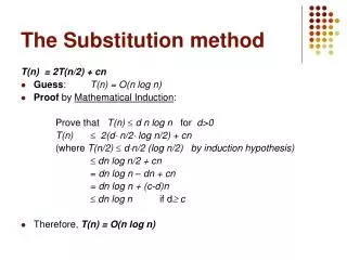
The Substitution method. T(n) = 2T(n/2) + cn Guess : T(n) = O(n log n) Proof by Mathematical Induction : Prove that T(n) d n log n for d>0 T(n) 2(d n/2 log n/2) + cn (where T(n/2) d n/2 (log n/2) by induction hypothesis) dn log n/2 + cn

The Substitution method
E N D
Presentation Transcript
The Substitution method T(n) = 2T(n/2) + cn • Guess: T(n) = O(n log n) • Proof by Mathematical Induction: Prove that T(n) d n log n for d>0 T(n)2(d n/2 log n/2) + cn (where T(n/2) dn/2 (log n/2) by induction hypothesis) dn log n/2 + cn = dn log n – dn + cn = dn log n + (c-d)n dn log n if d c • Therefore, T(n) = O(n log n)
Quick Sort – Partitioning – algorithm publicint partition(Comparable[] arr, int low, int high) { Comparable pivot = arr[high]; // choose pivot int l = low; int r = high-1; while (l<=r) { // find bigger item on the left while (l<=r && arr[l].compareTo(pivot) <= 0) l++; // find smaller item on the right while (l<=r && arr[r].compareTo(pivot) >= 0) r--; if (l<r) { swap(arr[l], arr[r]); l++; r--; } } // put pivot to the correct location swap(arr[l], arr[high]); return r; }
Quick Sort – Partitioning – algorithm – Proof of correctness • Loop invariant:at the beginning/end of each loop: • arr[low]..arr[l-1] contains elements <= pivot • arr[r+1]..arr[high-1] contains elements >= pivot • When the loop is finished we have l=r+1, i.e., • arr[low]..arr[r] are <= pivot • arr[r+1]..arr[high-1] are >= pivot • arr[high]=pivot • By swapping arr[high] with arr[l] (or arr[r]) we get a proper partitioning.
Quick Sort – Partitioning – another algorithm (textbook) • Pivot is chosen to be the first element of the array (does not really matter) • The array is divided to 4 parts (see bellow), initially “<p” and “¸p” parts are empty • Invariant for the partition algorithm: The items in region S1 are all less than the pivot, and those in S2 are all greater than or equal to the pivot • In each step the first element in “?” part is added either to “<p” or “¸p” part.
Quick Sort – Partitioning – another algorithm (textbook) S1: arr[first+1]..arr[lastS1] ) empty S2: arr[lastS1+1]..arr[firstUnknown-1] ) empty ?: arr[firstUnknown]..arr[last] ) all elements but pivot Initial state of the array
Quick Sort – Partitioning – another algorithm (textbook) Processing arr[firstUnknown]: case “< pivot” Move arr[firstUnknown] into S1 by swapping it with theArray[lastS1+1] and by incrementing both lastS1 and firstUnknown.
Quick Sort – Partitioning – another algorithm (textbook) Processing arr[firstUnknown]: case “¸ pivot” Moving theArray[firstUnknown] into S2 by incrementing firstUnknown.
Quick Sort – Partitioning – another algorithm (textbook) publicint partition(Comparable[] arr, int first, int last) { Comparable pivot = arr[first]; // choose pivot // initially everything but pivot is unknown int lastS1 = first; for (int firstUnknown = first+1; firstUnknown <= last; firstUnknown++) { if (arr[firstUnknown].compareTo(pivot) < 0) { // item should be moved to S1 lastS1++; swap(arr[lastS1],arr[firstUnknown]); } // else item should be moved to S2, // which will be increamenting firstUnknown in the loop } // put pivot to the correct location swap(arr[first], arr[lastS1]); return lastS1; }
Quick Sort – Selection of pivot • In the above algorithm we selected the pivot to be the last or the first element of subarray which we want to partition • It turns out that the selection of pivot is crucial for performance of Quick Sort – see best and worst cases • Other strategies used: • select 3 (or more elements) and pick the median • randomly select (especially used when the arrays might be originally sorted) • select an element “close to the median” in the subarray (there is a recursive linear time algorithm for that, see http://en.wikipedia.org/wiki/Selection_algorithm for details).
Analysis of Quick Sort:Best Case • How much time do we need to partition an array of size n? • O(n) using any of two algorithms • Best case: Suppose each partition operation divides the array almost exactly in half
Analysis of Quick Sort:Best Case • How much time do we need to partition an array of size n? • O(n) using any of two algorithms • Best case: Suppose each partition operation divides the array almost exactly in half • When could the best case happen? • For example, array was sorted and the pivot is selected to be the middle element of the subarray.
Analysis of Quick Sort:Best Case • Best case: Suppose each partition operation divides the array almost exactly in half • The running time (time cost) can be expressed with the following recurrence:T(n) = 2.T(n/2) + T(partitioning array of size n) = 2.T(n/2) + O(n) • The same recurrence as for merge sort, i.e., T(n) is of order O(n.log n).
Analysis of Quick Sort:Worst Case • In the worst case, partitioning always divides the sizenarray into these three parts: • A length one part, containing the pivot itself • A length zero part, and • A lengthn-1part, containing everything else
Analysis of Quick Sort:Worst Case • In the worst case, partitioning always divides the sizenarray into these three parts: • A length one part, containing the pivot itself • A length zero part, and • A lengthn-1part, containing everything else • When could this happen? • Example: the array is sorted and the pivot is selected to be the first or the last element.
Analysis of Quick Sort:Worst Case • The recurrent formula for the time cost of Quick Sort in the worst case:T(n) = T(0) + T(n-1) + O(n) = T(n-1) + O(n) • By repeated substitution (or Master’s theorem) we get the running time of Quick Sort in the worst case isO(n2) • Similar, situation as for Insertion Sort. Does it mean that the performance of Quick Sort is bad on average?
Quick Sort:Average Case • If the array is sorted to begin with, Quick sort running time is terrible: O(n2)(Remark: could be improved by random selection of pivot.) • It is possible to construct other bad cases • However, Quick sort runs usually (on average) in time O(n.log2n) -> CMPT307 for detailed analysis • The constant in front of n.log2n is so good that Quick sort is generally the fastest algorithm known. • Most real-world sorting is done by Quick sort.
Exercise Problem on Quick Sort. What is the running time of QUICKSORT when a) All elements of array A have the same value ? b) The array A contains distinct elements and in sorted decreasing order ?
Answer – 1st algorithm • Pivot is chosen to be the last element in the subarray. a) Whatever pivot you choose in each subarray it would result in WORST CASE PARTITIONING (l=high) and hence the running time is O(n2). b) Same is the case. Since you always pick the minimum element in the subarray as the pivot each partition you do would be a worst case partition and hence the running time is O(n2) again !
Answer – 2nd algorithm • Pivot is chosen to be the first element in the subarray a) Whatever pivot you choose in each subarray it would result in WORST CASE PARTITIONING (everything will be put to S2 part) and hence the running time is O(n2). b) Same is the case. Since you always pick the maximum element in the sub array as the pivot each partition you do would be a worst case partition and hence the running time is O(n2) again !
A Comparison of Sorting Algorithms Approximate growth rates of time required for eight sorting algorithms
Finding the k-th Smallest Element in an Array (Selection Problem) • One possible strategy: sort an array and just take the k-th element in the array • This would require O(n.log n) time if use some efficient sorting algorithm • Question: could we use partitioning idea (from Quicksort)?
Finding the k-th Smallest Element in an Array • Assume we have partition the subarray as before. If S1 contains k or more items -> S1 contains kth smallest item If S1 contains k-1 items -> k-th smalles item is pivot p If S1 contains fewer then k-1 items -> S2 contains kth smallest item
Finding the k-th Smallest Element in an Array public Comparable select(int k, Comparable[] arr, int low, int high) // pre: low <= high and // k <= high-low+1 (number of elements in the subarray) // return the k-th smallest element // of the subarray arr[low..high] { int pivotIndex = partition(arr, low, high); // Note: pivotIndex - low is the local index // of pivot in the subarray if (k == pivotIndex - low + 1) { // the pivot is the k-th element of the subarray return arr[pivotIndex]; } elseif (k < pivotIndex - low + 1) { // the k-th element must be in S1 partition return select(k, arr, low, pivotIndex-1); } else { // k > pivotIndex - low +1 // the k-th element must be in S2 partition // Note: there are pivotIndex-first elements in S1 // and one pivot, i.e., all smaller than // elements in S2, so we have to recalculate // index k return select(k - (pivotIndex-first+1), arr, pivotIndex+1, high); } } // end kSmall
Finding the k-th Smallest Item in an Array • The running time in the best case:T(n) = T(n/2) + O(n) • It can be shown with repeated substitution that T(n) is of order O(n) • The running time in the worst case:T(n) = T(n-1) + O(n) • This gives the time O(n2) • average case: O(n) • By selecting the pivot close to median (using a recursive linear time algorithm), we can achieve O(n) time in the worst case as well.