Understanding Arc Length Approximations in Calculus
0 likes | 16 Vues
Approximating the arc length of curves using calculus involves methods like measuring small straight lines and utilizing Pythagorean theorem. The formula for calculating arc length in Cartesian form is explored, along with examples demonstrating how to find arc length over specified intervals. Trigonometric substitutions and computer algebra systems are also discussed in the context of finding arc lengths for various functions.

Understanding Arc Length Approximations in Calculus
E N D
Presentation Transcript
Lengths of Curves: If we want to approximate the length of a curve, over a short distance we could measure a straight line. ds dy dx 2 dy dx 1 ds dx 2 By the pythagorean theorem: 2 2 2 ds dx dy 2 dy dx 1 s dx 2 2 2 ds dx dy 2 dy dx Length of Curve (Cartesian) 2 1 ds dx 2 2 dy dx b 1 s dx 2 dy dx 1 ds dx a 2
Arc Length Formula ( ) f x y ( ) g y x s s 2 2 dx dy dy dx d b 1 s dy 1 s dx c a General arc length formula . s ds
s ds ( ) g y x ( ) f x y 2 2 dx dy dy dx d b 1 s dy 1 s dx c a
Example: Find the arc length for the function over the specified interval. 0,5 . y x x 3/2, over s ds 2 2 dx dy dy dx d b 1 s dy 1 s dx c a 3 2 dy dx 1/2 s x 2 3 2 5 1/2 1 s x dx 0 9 4 5 1 s x dx 0
9 4 5 u Substitution 335 units = 12.407 units 27 1 s x dx 9 4 0 1 u x 4 9 49/4 1/2 s u du 9 4 du dx 1 (5,11.2) 4 2 9 3 49/4 4 9du u 3/2 s dx 1 3/2 New Bounds Lower Bound 8 27 49 4 1 3/2 s s 9 4 0 0 1 1 u 3 8 27 7 2 1 s Upper Bound 49 4 9 4 5 5 8 27 343 8 8 8 335 units 27 1 u s 2 2 5 11.2 12.265 units
Example: Find the arc length for the function over the specified interval. , over 0,4 . x y y s ds (2,4) 2 x y 2 dx dy dy dx d b 1 s dy 1 s dx s c a 1 2 dx dy 1/2 y 2 1 2 4 1/2 1 s y dy 0 1 4 4 1 1 s y dy 0
u 1 4 Substitution 2 2 Substituting we get tan u 1 4 1 4 1 4(tan 1 4 1) 4 1 1 s y dy 2 u y u y 0 2 1 2 u du dy 4 1 4sec 2 1 s dy 4 y 0 New Bounds Lower Bound 0 u Upper Bound 4 u 2 2 2 sec sec s d 1 4 1 2 y 1 4 4 s dy 0 0 2 y 2 sec sec s d 1 2 1 2 0 y 1 4 1 2 4 3 sec s d s dy 2 4 y 0 Trig Substitution 2 u 1 4 2 1 2 2 u du s Let tan u u 0 1 4 sec tan ln sec tan s 2 1 2 2 2 s u du 1 4 2 So sec du d 0 Now what? Obviously, Trig-Sub!!
1 4 sec tan ln sec tan s 1 2 (2,4) Recall tan u So tan 2u x y u 2 4 1 s 2u 1 2 1 4 1 2 1 2 2 2 4 ln 4 s u u u u 0 1 4 17 4 ln 17 0 0 4 s s 17 ln 17 4 units 1 4 Wow!!
Computer Algebra Systems 2 1 2 4 1/2 (2,4) 1 s y dy 0 s 4.472 units 2 2 2 4 s 17 ln 17 4 units 1 4 s 4.647 units
Example: Find the arc length for the function over the specified interval. sin , over 0, . y x x s ds 2 dy dx b 1 s dx s a No exact answer, just an approximation. dy dx cos x s 3.820 units 2 1 cos s x dx 0 F, the antiderivative, is not an elementary function.
Example: Find the arc length for the function over the specified interval. sin , over 0, . y x x s ds 2 dy dx b 1 s dx s a dy dx cos x 2 1 cos s x dx 0 F, the antiderivative, is not an elementary function.