Understanding Interval Estimation and T-Tests for Two Means
This comprehensive guide explores interval estimation and t-tests, including both independent and matched samples. We delve into the critical concepts of confidence intervals, hypothesis testing, and variance. The tutorial outlines how to determine confidently if the difference between two means (e.g., boys' and girls' scores) is statistically significant. Key formulas, assumptions, and methods for calculating the sampling distribution of difference between means are included, providing a solid foundation for statistical analysis in various fields.

Understanding Interval Estimation and T-Tests for Two Means
E N D
Presentation Transcript
Tuesday, October 22 • Interval estimation. • Independent samples t-test • for the difference between two means. • Matched samples t-test
Tuesday, October 23 • Interval estimation. • Independent samples t-test • for the difference between two means. • Matched samples t-test
Interval Estimation (a.k.a. confidence interval) Is there a range of possible values for that you can specify, onto which you can attach a statistical probability?
Interval Estimation (a.k.a. confidence interval) Is there a range of possible values for that you can specify, onto which you can attach a statistical probability?
Confidence Interval _ _ X - tsX X + tsX Where t = critical value of t for df = N - 1, two-tailed X = observed value of the sample _
Tuesday, October 23 • Interval estimation. • Independent samples t-test • for the difference between two means. • Matched samples t-test
Tuesday, October 22 • Interval estimation. • Independent samples t-test • for the difference between two means. • Matched samples t-test
H0 : 1 - 2 = 0 H1 : 1 - 2 0
_ _ Xgirls=51.16 Xboys=53.75 How do we know if the difference between these means, of 53.75 - 51.16 = 2.59, is reliably different from zero?
_ _ Xgirls=51.16 Xboys=53.75 We could find confidence intervals around each mean... 95CI: 52.07 boys 55.43 95CI: 49.64 girls 52.68
H0 : 1 - 2 = 0 H1 : 1 - 2 0 But we can directly test this hypothesis...
H0 : 1 - 2 = 0 H1 : 1 - 2 0 To test this hypothesis, you need to know … …the sampling distribution of the difference between means. - - X1-X2
H0 : 1 - 2 = 0 H1 : 1 - 2 0 To test this hypothesis, you need to know … …the sampling distribution of the difference between means. - - X1-X2 …which can be used as the error term in the test statistic.
X1-X2 = 2X1 +2X2 The sampling distribution of the difference between means. - - - - This reflects the fact that two independent variances contribute to the variance in the difference between the means.
X1-X2 = 2X1 +2X2 The sampling distribution of the difference between means. - - - - This reflects the fact that two independent variances contribute to the variance in the difference between the means. Your intuition should tell you that the variance in the differences between two means is larger than the variance in either of the means separately.
(X1 - X2) z = X1-X2 The sampling distribution of the difference between means, at n = , would be: - - - -
The sampling distribution of the difference between means. - - X1-X2 = 21 22 + n1n2 Since we don’t know , we must estimate it with the sample statistic s.
The sampling distribution of the difference between means. - - X1-X2 = 21 22 + n1n2 Rather than using s21 to estimate 21 and s22 to estimate 22 , we pool the two sample estimates to create a more stable estimate of 21 and 22 by assuming that the variances in the two samples are equal, that is, 21 = 22 .
sp2 sp2 sX1-X2 = + N1 N2
sp2 sp2 sX1-X2 = + N1 N2
SSw SS1 + SS2 sp2 = = N-2N-2 sp2 sp2 sX1-X2 = + N1 N2
(X1 - X2) - (1 - 2 ) t = sX1-X2 Because we are making estimates that vary by degrees of freedom, we use the t-distribution to test the hypothesis. …at (n1 - 1) + (n2 - 1) degrees of freedom (or N-2)
Assumptions • X1 and X2 are normally distributed. • Homogeneity of variance. • Samples are randomly drawn from their respective populations. • Samples are independent.