SCIENTIFIC DATA MANAGEMENT
SCIENTIFIC DATA MANAGEMENT. Arie Shoshani. Computational Research Division Lawrence Berkeley National Laboratory February , 2007. Outline. Problem areas in managing scientific data Motivating examples Requirements The DOE Scientific Data Management Center

SCIENTIFIC DATA MANAGEMENT
E N D
Presentation Transcript
SCIENTIFIC DATA MANAGEMENT Arie Shoshani Computational Research Division Lawrence Berkeley National Laboratory February , 2007
Outline • Problem areas in managing scientific data • Motivating examples • Requirements • The DOE Scientific Data Management Center • A three-layer architectural approach • Some results of technologies (details in mini-symposium) • Specific technologies from LBNL • Fastbit: innovative bitmap indexing for very large datasets • Storage Resource Managers: providing uniform access to storage systems
Motivating Example - 1 • Optimizing Storage Management and Data Accessfor High Energy and Nuclear Physics Applications # members # events/ year volume/year- Date of TB /institutions Experiment first data 350/35 8 9 STAR 2001 500 -10 10 350/35 9 PHENIX 2001 600 10 300/30 9 BABAR 1999 80 10 200/40 10 CLAS 1997 300 10 1200/140 10 ATLAS 2007 5000 10 STAR: Solenoidal Tracker At RHIC RHIC: Relativistic Heavy Ion Collider LHC: Large Hadron Collider Includes: ATLAS, STAR, … A mockup of An “event”
Typical Scientific Exploration Process • Generate large amounts of raw data • large simulations • collect from experiments • Post-processing of data • analyze data (find particles produced, tracks) • generate summary data • e.g. momentum, no. of pions, transverse energy • Number of properties is large (50-100) • Analyze data • use summary data as guide • extract subsets from the large dataset • Need to access events based on partialproperties specification (range queries) • e.g. ((0.1 < AVpT < 0.2) ^ (10 < Np < 20)) v (N > 6000) • apply analysis code
Motivating example - 2 • Combustion simulation: 1000x1000x1000 mesh with 100s of chemical species over 1000s of time steps – 1014 data values • Astrophysics simulation: 1000x1000x1000 mesh with 10s of variables per cell over 1000s of time steps - 1013 data values • This is an image of a single variable • What’s needed is search overmultiple variables, such as • Temperature > 1000AND pressure > 106AND HO2 > 10-7 AND HO2 > 10-6 • Combining multiple single-variable indexes efficiently is a challenge • Solution: specialized bitmap indexes
SRM Motivating Example - 3 • Earth System Grid Accessing large distributed stores for by 100’s of scientists • Problems • Different storage systems • Security procedures • File streaming • Lifetime of request • Garbage collection • Solution • Storage Resource Managers (SRMs)
M3D-L (Linear stability) XGC-ET Mesh/Interpolation Yes Stable? No Distributed Store M3D XGC-ET Mesh/Interpolation Distributed Store t Stable? B healed? No Mesh/Interpolation TBs Yes GBs Compute Puncture Plots Noise Detection Web-Portal (ElVis) Island detection Need More Flights? Distributed Store Blob Detection Feature Detection Out-of-core Isosurface methods MBs wide-area network Motivating Example 4: Fusion SimulationCoordination between Running Codes
Motivating example - 5 • Data Entry and Browsing tool for entering and linking metadata from multiple data sources • Metadata Problem for Microarray analysis • Microarray schemas are quite complex • Many objects: experiments, samples, arrays, hybridization, measurements, … • Many associations between them • Data is generated and processed in multiple locations which participate in the data pipeline • In this project: Synechococcus sp. WH8102 whole genome • microbes are cultured at Scripps Institution of Oceanography (SIO) • then the sample pool is sent to The Institute for Genomics Research (TIGR) • then images send to Sandia Lab for Hyperspectral Imaging and analysis • Metadata needs to be captured and LINKED • Generating specialized user interfaces is expensive and time-consuming to build and change • Data is collected on various systems, spreadsheets, notebooks, etc.
1) The microbes are cultured at SIO 2) Microarray hybridization at TIGR HS_Experiment Link From TIGR to SIO Nucleotide Pool 3) Hyperspectral imaging at Sandia Link to MA-Scan HS_Slide Probe Source HS-Scan MA-Scan Probe MCR-Analysis Analysis probe1 probe2 Study Hybridization Slide LCS-Analysis The kind of technology needed DEB: Data Entry and Browsing Tool • Features - Interface based on lab notebook look and feel - Tools are built on top of commercial DBMS - Schema-driven automatic Screen generation
Storage Growth is Exponential • Unlike compute and network resources, storage resources are not reusable • Unless data is explicitly removed • Need to use storage wisely • Checkpointing, remove replicated data • Time consuming, tedious tasks • Data growth scales with compute scaling • Storage will grow even with good practices (such as eliminating unnecessary replicas) • Not necessarily on supercomputers but, on user/group machines and archival storage • Storage cost is a consideration • Has to be part of science growth cost • But, storage costs going down at a rate similar to data growth • Need continued investment in new storage technologies Storage Growth 1998-2006 at ORNL (rate: 2X / year) Storage Growth 1998-2006 at NERSC-LBNL (rate: 1.7X / year) The challenges are in managing the data
Data and Storage ChallengesEnd-to-End: 3 Phases of Scientific Investigation) • Data production phase • Data movement • I/O to parallel file system • Moving data out of supercomputer storage • Sustain data rates of GB/sec • Observe data during production • Automatic generation of metadata • Post-processing phase • Large-scale (entire datasets) data processing • Summarization / statistical properties • Reorganization / transposition • Generate data at different granularity • On-the-fly data processing • computations for visualization / monitoring • Data extraction / analysis phase • Automate data distribution / replication • Synchronize replicated data • Data lifetime management to unclog storage • Extract subsets efficiently • Avoid reading unnecessary data • Efficient indexes for “fixed content” data • Automated use of metadata • Parallel analysis tools • Statistical analysis tools • Data mining tools
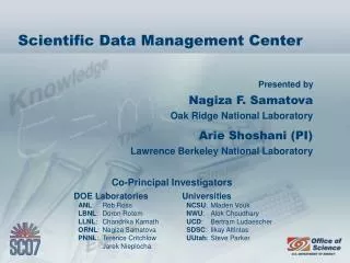
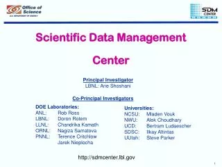
The Scientific Data Management Center (Center for Enabling Technologies - CET) • PI: Arie Shoshani, LBNL • Annual budget: 3.3 Million • Established 5 years ago (SciDAC-1) • Successfully re-competed for the next 5 years (SciDAC-2) • Featured in second issue of SciDAC magazine • Laboratories • ANL, ORNL, LBNL, LLNL, PNNL • Universities • NCSU, NWU, SDSC, UCD, Uof Utah, http://www.scidacreview.org/0602/pdf/data.pdf
Tapes Disks Disks Tapes Scientific Data Management Center Petabytes Petabytes Scientific Simulations & experiments Terabytes Terabytes • Climate Modeling • Astrophysics • Genomics and Proteomics • High Energy Physics • Fusion… SDM-ISIC Technology • Optimizing shared access from mass storage systems • Parallel-IO for various file formats • Feature extraction techniques • High-dimensional cluster analysis • High-dimensional indexing • Parallel statistics • … Data Manipulation: Data Manipulation: ~20% time • Using SDM-Center technology • Getting files from Tape archive • Extracting subset of data from files • Reformatting data • Getting data from heterogeneous, distributed systems • moving data over the network ~80% time Scientific Analysis & Discovery ~80% time Scientific Analysis & Discovery ~20% time Current Goal
A Typical SDM Scenario Task A: Generate Time-Steps Task B: Move TS Task D: Visualize TS Task C: Analyze TS Control Flow Layer + Flow Tier Applications & Software Tools Layer Data Mover Post Processing Parallel R Terascale Browser Simulation Program Work Tier I/O System Layer Subset extraction File system HDF5 Libraries Parallel NetCDF PVFS SRM Storage & Network Resouces Layer
Approach SDM Framework • Use an integrated framework that: • Provides a scientific workflow capability • Supports data mining and analysis tools • Accelerates storage and access to data • Simplify data management tasks for the scientist • Hide details of underlying parallel and indexingtechnology • Permit assembly of modules using a simple graphical workflow description tool Scientific Process Automation Layer Data Mining & Analysis Layer Scientific Application Scientific Understanding Storage Efficient Access Layer
Technology Details by Layer Scientific Scientific Scientific Workflow Components Web WorkFlow WorkFlow Process Process Wrapping Management Management Automation Automation Tools Engine Tools (SPA) (SPA) Layer Layer Data Data Data Analysis and Feature Identification Efficient Efficient ASPECT: Data Efficient Efficient Parallel R Mining & Mining & indexing indexing integration Analysis Parallel Parallel Statistical Analysis Analysis (Bitmap (Bitmap Framework tools Visualization Visualization Analysis Index) Index) (PCA, ICA) ( ( pVTK pVTK ) ) (DMA) (DMA) Layer Layer Storage Storage Parallel Parallel Parallel ROMIO Storage Storage Parallel Parallel Efficient Efficient Virtual Virtual MPI I/O - IO Resource Resource NetCDF NetCDF Access Access File File System Manager Manager (SRM) (ROMIO) System System (SEA) (SEA) (To HPSS) Layer Layer Hardware, OS, and MSS (HPSS) Hardware, OS, and MSS (HPSS)
Technology Details by Layer Scientific Scientific Scientific Workflow Components Web WorkFlow WorkFlow Process Process Wrapping Management Management Automation Automation Tools Engine Tools (SPA) (SPA) Layer Layer Data Data Data Analysis and Feature Identification Efficient Efficient ASPECT: Data Efficient Efficient Parallel R Mining & Mining & indexing indexing integration Analysis Parallel Parallel Statistical Analysis Analysis (Bitmap (Bitmap Framework tools Visualization Visualization Analysis Index) Index) (PCA, ICA) ( ( pVTK pVTK ) ) (DMA) (DMA) Layer Layer Storage Storage Parallel Parallel Parallel ROMIO Storage Storage Parallel Parallel Efficient Efficient Virtual Virtual MPI I/O - IO Resource Resource NetCDF NetCDF Access Access File File System Manager Manager (SRM) (ROMIO) System System (SEA) (SEA) (To HPSS) Layer Layer Hardware, OS, and MSS (HPSS) Hardware, OS, and MSS (HPSS)
Data Generation Scientific Process Automation Layer Workflow Design and Execution SimulationRun Data Mining and Analysis Layer ParallelnetCDF MPI-IO PVFS2 Storage Efficient Access Layer OS, Hardware (Disks, Mass Store)
P0 P1 P2 P3 netCDF Parallel File System P0 P1 P2 P3 Parallel netCDF Parallel File System Parallel NetCDF v.s. HDF5 (ANL+NWU) Interprocess communication Parallel Virtual File System: Enhancements and deployment • Developed Parallel netCDF • Enables high performance parallel I/O to netCDF datasets • Achieves up to 10 fold performance improvement over HDF5 • Enhanced ROMIO: • Provides MPI access to PVFS2 • Advanced parallel file system interfaces for more efficient access • Developed PVFS2 • Production use at ANL, Ohio SC, Univ. of Utah HPC center • Offered on Dell clusters • Being ported to IBM BG/L system After Before FLASH I/O Benchmark Performance (8x8x8 block sizes)
Technology Details by Layer Scientific Scientific Scientific Workflow Components Web WorkFlow WorkFlow Process Process Wrapping Management Management Automation Automation Tools Engine Tools (SPA) (SPA) Layer Layer Data Data Data Analysis and Feature Identification Efficient Efficient ASPECT: Data Efficient Efficient Parallel R Mining & Mining & indexing indexing integration Analysis Parallel Parallel Statistical Analysis Analysis (Bitmap (Bitmap Framework tools Visualization Visualization Analysis Index) Index) (PCA, ICA) ( ( pVTK pVTK ) ) (DMA) (DMA) Layer Layer Storage Storage Parallel Parallel Parallel ROMIO Storage Storage Parallel Parallel Efficient Efficient Virtual Virtual MPI I/O - IO Resource Resource NetCDF NetCDF Access Access File File System Manager Manager (SRM) (ROMIO) System System (SEA) (SEA) (To HPSS) Layer Layer Hardware, OS, and MSS (HPSS) Hardware, OS, and MSS (HPSS)
Statistical Computing with R • About R (http://www.r-project.org/): • R is an Open Source (GPL), most widely used programming environment for statistical analysis and graphics; similar to S. • Provides good support for both users and developers. • Highly extensible via dynamically loadable add-on packages. • Originally developed by Robert Gentleman and Ross Ihaka. > … > dyn.load( “foo.so”) > .C( “foobar” ) > dyn.unload( “foo.so” ) > library(mva) > pca <- prcomp(data) > summary(pca) > library (rpvm) > .PVM.start.pvmd () > .PVM.addhosts (...) > .PVM.config ()
Task-parallel analyses: Data-parallel analyses: • Likelihood Maximization. • Re-sampling schemes: Bootstrap, Jackknife, etc. • Animations • Markov Chain Monte Carlo (MCMC). • Multiple chains. • Simulated Tempering: running parallel chains at different “temperature“ to improve mixing. • k-means clustering • Principal Component Analysis (PCA) • Hierarchical (model-based) clustering • Distance matrix, histogram, etc. computations Providing Task and Data Parallelism in pR
Parallel R (pR) Distribution http://www.ASPECT-SDM.org/Parallel-R • Releases History: • pR enables both data and task parallelism (includes task-pR and RScaLAPACK) (version 1.8.1) • RScaLAPACK provides R interface to ScaLAPACK with its scalability in terms of problem size and number of processors using data parallelism (release 0.5.1) • task-pR achieves parallelism by performing out-of-order execution of tasks. With its intelligent scheduling mechanism it attains significant gain in execution times (release 0.2.7) • pMatrix provides a parallel platform to perform major matrix operations in parallel using ScaLAPACK and PBLAS Level II & III routines • Also: Available for download from R’s CRAN web site (www.R-Project.org) with 37 mirror sites in 20 countries
Technology Details by Layer Scientific Scientific Scientific Workflow Components Web WorkFlow WorkFlow Process Process Wrapping Management Management Automation Automation Tools Engine Tools (SPA) (SPA) Layer Layer Data Data Data Analysis and Feature Identification Efficient Efficient ASPECT: Data Efficient Efficient Parallel R Mining & Mining & indexing indexing integration Analysis Parallel Parallel Statistical Analysis Analysis (Bitmap (Bitmap Framework tools Visualization Visualization Analysis Index) Index) (PCA, ICA) ( ( pVTK pVTK ) ) (DMA) (DMA) Layer Layer Storage Storage Parallel Parallel Parallel ROMIO Storage Storage Parallel Parallel Efficient Efficient Virtual Virtual MPI I/O - IO Resource Resource NetCDF NetCDF Access Access File File System Manager Manager (SRM) (ROMIO) System System (SEA) (SEA) (To HPSS) Layer Layer Hardware, OS, and MSS (HPSS) Hardware, OS, and MSS (HPSS)
Piecewise Polynomial Models for Classification of Puncture (Poincaré) plots • Classify each of the nodes: quasiperiodic, islands, separatrix • Connections between the nodes • Want accurate and robust classification, valid when few points in each node National Compact Stellarator Experiment Quasiperiodic Islands Separatrix
Polar Coordinates • Transform the (x,y) data to Polar coordinates (r,). • Advantages of polar coordinates: • Radial exaggeration reveals some features that are hard to see otherwise. • Automatically restricts analysis to radial band with data, ignoring inside and outside. • Easy to handle rotational invariance.
Piecewise Polynomial Fitting: Computing polynomials • In each interval, compute the polynomial coefficients to fit 1 polynomial to the data. • If the error is high, split the data into an upper and lower group. Fit 2 polynomials to the data, one to each group. Blue: data.Red: polynomials. Black: interval boundaries.
Classification • The number of polynomials needed to fit the data and the number of gaps gives the information needed to classify the node: 2 Polynomials 2 Gaps Islands 2 Polynomials 0 Gaps Separatrix
Technology Details by Layer Scientific Scientific Scientific Workflow Components Web WorkFlow WorkFlow Process Process Wrapping Management Management Automation Automation Tools Engine Tools (SPA) (SPA) Layer Layer Data Data Data Analysis and Feature Identification Efficient Efficient ASPECT: Data Efficient Efficient Parallel R Mining & Mining & indexing indexing integration Analysis Parallel Parallel Statistical Analysis Analysis (Bitmap (Bitmap Framework tools Visualization Visualization Analysis Index) Index) (PCA, ICA) ( ( pVTK pVTK ) ) (DMA) (DMA) Layer Layer Storage Storage Parallel Parallel Parallel ROMIO Storage Storage Parallel Parallel Efficient Efficient Virtual Virtual MPI I/O - IO Resource Resource NetCDF NetCDF Access Access File File System Manager Manager (SRM) (ROMIO) System System (SEA) (SEA) (To HPSS) Layer Layer Hardware, OS, and MSS (HPSS) Hardware, OS, and MSS (HPSS)
Example Data Flow in Terascale Supernova Initiative Logistical Network Courtesy: John Blondin
Original TSI Workflow Examplewith John Blondin, NCSU Automate data generation, transfer and visualization of a large-scale simulation at ORNL
Node Retrieve File from XRaid Node-0 Node-1 ….. Node-21 Top level TSI Workflow Automate data generation, transfer and visualization of a large-scale simulation at ORNL Check whether a time slice is finished Submit Job to Cray at ORNL Aggregate all into One large File - Save to HPSS Yes Yes Split it into 22 Files and store them in XRaid ORNL NCSU Head Node submit scheduling to SGE Notify Head Node at NC State SGE schedule the transfer for 22 Nodes Start Ensight to generate Video Files at Head Node
Using the Scientific Workflow Tool (Kepler)Emphasizing Dataflow (SDSC, NCSU, LLNL) Automate data generation, transfer and visualization of a large-scale simulation at ORNL
New actors in Fusion workflowto support automated data movement KEPLER Start Two Independent processes Login At ORNL (OTP) Detect when Files are Generated Move files Tar files Archive files 2 Kepler Workflow Engine 1 Simulation Program (MPI) OTP Login actor File Watcher actor Scp File copier actor Tar’ing actor Local archiving actor Software components Disk Cache Disk Cache Hardware + OS HPSS ORNL Seaborg NERSC Disk cacke Ewok-ORNL
Re-applying Technology Technology Parallel NetCDF Parallel VTK Compressed bitmaps Storage Resource Managers Feature Selection Scientific Workflow SDM technology, developed for one application, can be effectively targeted at many other applications … Initial Application Astrophysics Astrophysics HENP HENP Climate Biology New Applications Climate Climate Combustion, Astrophysics Astrophysics Fusion (exp. & simulation) Astrophysics
Broad Impact of the SDM Center… Astrophysics: High speed storage technology, parallel NetCDF, integration software used for Terascale Supernova Initiative (TSI) and FLASH simulations Tony Mezzacappa – ORNL, Mike Zingale – U of Chicago, Mike Papka – ANL Scientific Workflow John Blondin – NCSU Doug Swesty, Eric Myra – Stony Brook Climate: High speed storage technology, Parallel NetCDF, and ICA technology used for Climate Modeling projects Ben Santer – LLNL, John Drake – ORNL, John Michalakes – NCAR Combustion: Compressed Bitmap Indexing used for fast generation of flame regions and tracking their progress over time Wendy Koegler, Jacqueline Chen – Sandia Lab ASCI FLASH – parallel NetCDF Dimensionality reduction Region growing
Broad Impact (cont.) Biology: Kepler workflow system and web-wrapping technology used for executing complex highly repetitive workflow tasks for processing microarray data Matt Coleman - LLNL High Energy Physics: Compressed Bitmap Indexing and Storage Resource Managers used for locating desired subsets of data (events) and automatically retrieving data from HPSS Doug Olson - LBNL, Eric Hjort – LBNL, Jerome Lauret - BNL Fusion: A combination of PCA and ICA technology used to identify the key parameters that are relevant to the presence of edge harmonic oscillations in a Tokomak Keith Burrell - General Atomics Scott Klasky - PPPL Building a scientific workflow Dynamic monitoring of HPSS file transfers Identifying key parametersfor the DIII-D Tokamak
Technology Details by Layer Scientific Scientific Scientific Workflow Components Web WorkFlow WorkFlow Process Process Wrapping Management Management Automation Automation Tools Engine Tools (SPA) (SPA) Layer Layer Data Data Data Analysis and Feature Identification Efficient Efficient ASPECT: Data Efficient Efficient Parallel R Mining & Mining & indexing indexing integration Analysis Parallel Parallel Statistical Analysis Analysis (Bitmap (Bitmap Framework tools Visualization Visualization Analysis Index) Index) (PCA, ICA) ( ( pVTK pVTK ) ) (DMA) (DMA) Layer Layer Storage Storage Parallel Parallel Parallel ROMIO Storage Storage Parallel Parallel Efficient Efficient Virtual Virtual MPI I/O - IO Resource Resource NetCDF NetCDF Access Access File File System Manager Manager (SRM) (ROMIO) System System (SEA) (SEA) (To HPSS) Layer Layer Hardware, OS, and MSS (HPSS) Hardware, OS, and MSS (HPSS)
FastBit:An Efficient Indexing Technology For Accelerating Data Intensive Science Outline Overview Searching Technology Applications http://sdm.lbl.gov/fastbit
Searching Problems in Data Intensive Sciences • Find the collision events with the most distinct signature of Quark Gluon Plasma • Find the ignition kernels in a combustion simulation • Track a layer of exploding supernova These are not typical database searches: • Large high-dimensional data sets (1000 time steps X 1000 X 1000 X 1000 cells X 100 variables) • No modification of individual records during queries, i.e., append-only data • Complex questions: 500 < Temp < 1000 && CH3 > 10-4 && … • Large answers (hit thousands or millions of records) • Seek collective features such as regions of interest, beyond typical average, sum
Common Indexing Strategies Not Efficient Task: searching high-dimensional append-only data with ad hoc range queries • Most tree-based indices are designed to be updated quickly • E.g. family of B-Trees • Sacrifice search efficiency to permit dynamic update • Hash-based indices are • Efficient for finding a small number of records • But, not efficient for ad hoc multi-dimensional queries • Most multi-dimensional indices suffer curse of dimensionality • E.g. R-tree, Quad-trees, KD-trees, … • Don’t scale to high dimensions (< 20) • Are inefficient if some dimensions are not queried
Our Approach: An Efficient Bitmap Index • Bitmap indices • Sacrifice update efficiency to gain more search efficiency • Are efficient for multi-dimensional queries • Scale linearly as the number of dimensions actually used in a query • Bitmap indices may demand too much space • We solve the space problem by developing an efficient compression method that • Reduces the index size, typically 30% of raw data, vs. 300% for some B+-tree indices • Improves operational efficiency, 10X speedup • We have applied FastBit to speed up a number of DOE funded applications
FastBit In a Nutshell • FastBit is designed to search multi-dimensional append-only data • Conceptually in table format • rows objects • columns attributes • FastBit uses vertical (column-oriented) organization for the data • Efficient for searching • FastBit uses bitmap indices with a specializedcompression method • Proven in analysis to be optimal for single-attribute queries • Superior to others because they are also efficient for multi-dimensional queries column row
Column 2 Column 1 column n 0 0 0 0 0 0 0 0 0 0 0 0 0 0 0 0 0 0 0 1 0 0 0 1 0 0 0 0 0 0 0 0 0 0 0 1 1 1 0 1 1 1 0 1 1 1 0 1 1 0 0 0 0 0 0 0 0 0 0 0 0 1 0 0 0 0 0 0 0 0 0 0 0 0 0 0 0 0 0 0 0 0 0 0 0 0 0 1 0 0 0 0 0 0 0 0 0 0 0 0 0 0 0 0 0 0 0 0 0 0 1 1 1 0 1 1 1 0 1 1 1 0 1 1 0 0 0 0 0 0 0 0 0 0 0 0 1 0 0 0 0 0 0 1 0 0 0 0 0 0 0 0 0 0 0 0 0 0 0 0 0 0 1 0 0 0 0 0 0 0 0 0 0 0 0 0 0 0 0 0 0 0 0 0 1 0 0 0 0 0 0 0 0 0 0 0 0 0 0 0 0 0 0 0 0 0 0 0 0 0 0 0 0 0 0 0 0 0 1 0 0 0 0 0 0 0 0 0 0 0 1 1 1 0 1 1 1 0 1 1 1 0 1 1 0 0 0 0 0 0 0 0 0 0 0 0 1 0 0 0 0 0 0 0 0 0 0 0 0 0 0 0 0 0 0 0 0 0 0 0 0 0 1 0 0 0 0 0 0 0 0 0 0 0 0 0 0 0 0 0 . . . Bit-Sliced Index • Take advantage that index need to be is append only • partition each property into bins • (e.g. for 0<Np<300, have 300 equal size bins) • for each bin generate a bit vector • compress each bit vector (some version of run length encoding)
Basic Bitmap Index Data values • First commercial version • Model 204, P. O’Neil, 1987 • Easy to build: faster than building B-trees • Efficient for querying: only bitwise logical operations • A < 2 b0 OR b1 • A > 2 b3 OR b4 OR b5 • Efficient for multi-dimensional queries • Use bitwise operations to combine the partial results • Size: one bit per distinct value per object • Definition: Cardinality == number of distinct values • Compact for low cardinality attributes only, say, < 100 • Need to control size for high cardinality attributes b0 b1 b2 b3 b4 b5 1 0 0 0 0 0 1 0 0 0 1 0 0 1 0 0 0 1 0 0 0 0 0 1 0 0 0 0 0 0 1 0 0 0 0 0 0 0 0 0 0 0 0 1 0 0 0 1 0 0 0 0 0 0 0 1 5 3 1 2 0 4 1 =0 =1 =2 =3 =4 =5 A < 2 2 < A
Run Length Encoding • Uncompressed: • 0000000000001111000000000 ......0000001000000001111100000000 .... 000000 • Compressed: • 12, 4, 1000,1,8, 5,492 • Practical considerations: • Store very short sequences as-is (literal words) • Count bytes/words rather than bits (for long sequences) • Use first bit for type of word: literal or count • Use second bit of count to indicate 0 or 1 sequence • [literal] [31 0-words] [literal] [31 0-words] • [00 0F 00 00] [80 00 00 1F] [02 01 F0 00] [80 00 00 0F] • Other ideas • repeated byte patterns, with counts • - Well-known method use in Oracle: Byte-aligned Bitmap Code (BBC) Advantage: Can perform logical operations such as: AND, OR, NOT, XOR, … And COUNT operations directly on compressed data
FastBit Compression Method is Compute-Efficient Example: 2015 bits 10000000000000000000011100000000000000000000000000000……………….00000000000000000000000000000001111111111111111111111111 Main Idea: Use run-length-encoding, but... partition bits into 31-bit groups on 32-bit machines 31 bits 31 bits … 31 bits Merge neighboring groups with identical bits Count=63 (31 bits) 31 bits 31 bits Encode each group using one word • Name: Word-Aligned Hybrid (WAH) code (US patent 6,831,575) • Key features: WAH is compute-efficient because it • Uses the run-length encoding (simple) • Allows operations directly on compressed bitmaps • Never breaks any words into smaller pieces during operations
Compute Efficient Compression Method:10 times faster than best-known method 10X selectivity
A range Bitmaps in an index Time to Evaluate a Single-Attribute Range Condition in FastBit is Optimal • Evaluating a single attribute range condition may require OR’ing multiple bitmaps • Both analysis and timing measurement confirm that the query processing time is at worst proportional to the number of hits Worst case: Uniform Random Data Realistic case: Zipf Data BBC: Byte-aligned Bitmap Code The best known bitmap compression
Processing Multi-Dimensional Queries 1 0 0 0 0 0 1 0 0 0 1 0 0 1 0 0 0 1 0 0 0 0 0 1 0 0 0 0 0 0 1 0 0 0 0 0 0 0 0 0 0 0 0 1 0 0 0 1 0 0 0 0 0 0 1 0 0 0 0 0 1 0 0 0 0 0 0 0 0 0 0 1 0 0 1 0 0 1 0 0 0 0 0 0 0 0 0 0 0 0 0 0 0 0 1 0 0 1 0 0 1 0 1 0 0 0 0 0 • Merging results from tree-based indices is slow • Because sorting and merging are slow • Merging results from bitmap indices is fast • Because bitwise operations on bitmaps are efficient Fast slow 1 1 0 0 1 0 1 0 1 0 1 0 1 1 0 0 1 0 OR OR 2,4,5,8 1,2,5,7,9 2,5 AND 0 1 0 0 1 0 0 0 0