Download
1 / 86
890 likes | 1.15k Vues
An Introduction to Statistics. A Biologist – A Physicist who doesn’t like maths. Purpose of Statistics (1). Summarise Data Central tendency e.g. mean, median or mode Spread of data e.g. variance, standard deviation

E N D
An Introduction to Statistics A Biologist – A Physicist who doesn’t like maths
Purpose of Statistics (1) • Summarise Data • Central tendency e.g. mean, median or mode • Spread of data e.g. variance, standard deviation • These parameters can be used to abstract information from large or complex sets of data • Statistics simplify data
Purpose of Statistics (2) Compare Data Are male 1st year Biology students taller or shorter than male 1st year Physics students? Measure height of 20 students in each group Does any difference we see between the samples reflect a true difference in the entire population of both groups? What is the probability that the observed difference arose simply by chance (sampling error)?
Probability Probability is the chance of something happening Probability is essentially intuitive E.g. what is the probability (chance) of rolling a 2 using a standard 6-sided die Success = the outcome we are interested in (a 2) Outcomes = the total number of possible outcomes (6) Probability (P) = # Success = 1 # Outcomes 6
More Simple Probability ♠ ♣ ♥ ♦ 4 suits (2 black, 2 red) 13 cards per suit 3 ‘Court’ cards per suit Jack Queen King P(7) = 4 P(red 7) = 2 52 52 P(black card) = 26 = 1P(black Court card) = 6 52 2 52
The Probability Scale 0% 50% 100% 0 0.5 1 Impossible Evens Certain ‘Death and taxes’ P(4♥) = 1/52 = 1.92% = 0.0192 P(♠) = 13/52 = 25% = 0.25 P(Q) = 4/52 = 7.69% = 0.0769 Typically it is the 0 to 1 scale that is used in statistics
A Priori? We can work out the true probability (P) of rolling a number or picking a card because we understand the underlying process Randomly pick one card from a pack of 52 each of which has an equal chance of being picked This is call a priori knowledge But what if we don’t understand the underlying process?
Estimating Probabilities (P) You are given a bag of 1000 flower seeds, some of which will produce red flowers and some yellow. What is the probability of getting a yellow flower? You don’t know the underlying mechanism so plant a sample, see what proportion are yellow and estimate the probability (P) P = # successes = # yellow flowered plants # trials # seeds sown Estimated probability
Estimating Probabilities – Sample Size Let’s say that in the bag of 1000 seeds, 350 will produce yellow flowered-plants (P = 35/100) = 0.35 If you sow only 20, you could, conceivably, pick 20 yellow seeds. This apparent bias becomes less likely the more seeds you sow The larger the sample size the better the estimate
Randomness The yellow flower example depends upon a key characteristic of our sampling: Sampling MUST be RANDOM If sampling is non-random we cannot base our estimate of P on the # success/# trials We would have to factor into the equation the probability of picking a yellow seed out of the bag A failure to ensure that sampling is random renders simple interpretation of data invalid
Mendel’s Peas a priori P = 0.75 P = 0.74 From data
Complex Probability - OR What is the P for two (or more) events the P for each of which is not dependent on P for the other? What is the P of rolling a 3 or a 5 using an unbiased 6-side die? The answer is the sum of the P for each individual event P(3) = 1/6 = 0.167 P(5) = 1/6 = 0.167 P(3 OR 5) = 0.167 + 0.167 = 0.333 This should be intuitive – you’ve increased the range of successes whilst keeping the number of possible outcomes the same
More OR P(♥ OR 3) = 13/52 + 4/52 = 0.25 + 0.077 P(Court card or A) = 12/52 + 4/52 = 0.23 + 0.077 = 0.31 Going back to Mendel’s peas – what is the P for getting a tall plant in the heterozygote F1 cross progeny (F2)? Each combination has an equal P P(TT) = P(Tt) = P(Tt) = P(tt) = 0.25 P(tall) = P(TT OR Tt OR Tt) = 0.25 + 0.25 + 0.25 = 0.75 OR = SUM individual P
Complex Probability - AND Is the probability of rolling a double 1 less or greater than rolling a 1 with a single die? If you’ve ever played a board game like Monopoly you’ll have a feeling for the answer – doubles are ‘special’ because they have a low probability The overall probability depends on both events happening P(1 AND 1) = P(1) x P(1) = 1/6 x 1/6 = 0.1762 = 0.0278 When the overall success is dependent on several events you multiply the probabilities of the events Is P different if you roll one die twice or two dice once?
More AND In the following examples, two packs of cards are used. What is the probability of picking a 5 from one pack AND a red card from the second pack? P(5 AND red) = 4/52 x 26/52 = 0.077 x 0.5 = 0.038 P(♦ AND Court card) = 13/52 x 12/52 = 0.25 x 0.23 = 0.0577 P((J OR red) AND (Court OR ♣)) = (4/52 + 26/52) x (12/52 + 13/52) = (0.077 + 0.5) x (0.23 + 0.25) = 0.577 x 0.48 = 0.277 AND = Multiply Ps
Card Sharps A Royal Flush is a hand of cards containing the A, K, Q J and 10(T) all of the same suit. What is the P of dealing a Royal Flush (in any suit)? This problem is less simple than it first appears This problem is less difficult than it appears (after a little thought) It illustrates that there is nothing esoteric about probability – it’s all about thinking things through logically
Card Sharps – The 1st Card Problem We haven’t specified either the suit or the order in which the cards are to be dealt This means that the first card can be any AKQJT from any suit Therefore the P for the first card is 20/52 = 0.385 However, once you have dealt the first card, the remaining cards must come from the same suit Let’s imagine we deal A♥ as our 1st card
Card Sharps – Completing the Flush We’ve dealt A♥ so the remaining cards must also be ♥s The next card can be a KQJ or T of ♥P = 4/51 (deal = K♥) The next card can be QJ or T of ♥P = 3/50 (deal = Q♥) J or T of ♥P = 2/49 (deal = J♥) The last card has to be T♥P = 1/48 Therefore P(Royal Flush any suit) = 20/52 x 4/51 x 3/50 x 2/49 x 1/48 = 0.385 x 0.078 x 0.060 x 0.041 x 0.021 = 0.0000016 Notice each time we deal a card the possible outcomes reduce (we are not replacing the card in the pack) = 1 in 644600!
More Peas Norma? Mendel studied a number of unlinked traits: Tall dominant over dwarf P(Tall) = 0.75 (in F2) Round dominant over wrinkled P(Round) = 0.75 P for all outcomes must = 1 P(dwarf) = P(wrinkled) = 0.25 P(Tall AND Round) = 0.752 = 0.562 P(Dwarf AND wrinkled) = 0.252 = 0.0625 P(Tall AND Wrinkled) = 0.75 x 0.25 = 0.1875 P(Dwarf AND Round) = 0.25 x 0.75 = 0.1875 0.562 + 2(0.1875) + 0.0625 = 1.0 What is more 0.562/0.0625 = 9 and 0.1875/0.0625 = 3
Dihybrid Inheritance Cross homozygous tall round (TTRR) with homozygous dwarf wrinkled (ttrr) F1 heterozygotes = TtRr gametes TR, Tr, tR, tr F2 Tall Round (9) Tall Wrinkled (3) Dwarf Round (3) Dwarf Wrinkled (1)
Conditional Probability What is P of a 2 showing given that the die is showing an even number? P(2) = 1/6 = 0.167 In this case one success out of six possible outcomes (1,2,3,4,5, 6), but… P(2|even) = 1/3 = 0.333 In this case there are now only three possible outcomes (2,4,6)
Independence In the previous example whether the die showed a 2 was (obviously) dependent upon the die showing an even number But whether or not a die (die A) shows 2 does NOT depend on whether a second die (die B) shows even 2 on die A is independent of even on die B P(A shows 2|B shows even) = P(A shows 2) = 1/6 Independence means that P(A|B) = P(A) In general P(A|B) P(B|A) Thus, P(B shows even|A shows 2) = 3/6
Independence for Peas P(Round) = 423/556 = 0.761 P(Round|Yellow) = 315/416 = 0.757 P(Round|Green) = 108/140 = 0.771 P(Round) P(Round|Yellow) P(Round|Green) 0.75 traits for colour and seed shape are independent
Probability Summary P measured on scale 0 to 1 where 1 = certainty If there are n possible outcomes then P for one outcome = 1/n P of an event not happening = 1 – P(event) P(A OR B) = P(A) + P(B) (OR = Add) P(A AND B) = P(A) x P(B) (AND = multiply)
Regular (≠ Random) Random Biased Randomness Randomness is an important concept Most statistics and associated analyses require unbiased sampling Imagine placing quadrats in a field…
Creating Randomness Not as easy as you may think Rolling dice is fine – but limited Random number generators aren’t really random Tables of random numbers exist Beware of unintentional bias Two runs of a program designed to generate ‘random’ numbers!
Distributions Distributions describe the frequency with which individual events occur within a range of possible events As such, they are dependent on the P that a given event will occur There are a number of distributions, of which… The Normal (Gaussian) Distribution The Poisson Distribution The Binomial Distribution …are most relevant in a biological context
The Normal Distribution Continuous variate Typically results from a number of underlying causes e.g. height – depends on genome and environment First described by C. F. Gauss in 1809 (hence Gaussian) Sometimes (erroneously) described as parametric
The Normal Distribution - Example Weight (mg) crickets (adapted from Gould and Gould, 2002)
Line approximates to normal distribution The Normal Distribution - Example
The Normal Distribution – Caution! Larger sample size Smaller interval size Smaller sample size Larger interval size In statistics, size matters Big is beautiful
The Normal Distribution When n , andinterval 0 then…. This is the ‘bell-shaped’ Normal Distribution
The Mean m – population mean Reads – the sum (S) of all observations (x) from 1 to N (number of observations), divided by N
The Normal Distribution and P The mean (m) is a measure of central tendency m P P When sampling, the P of obtaining a value close to m is greater than P for values distant from m
The Effect of Sample Size The larger the sample size, the more accurately it reflects the underlying distribution In the following example, the red bars are the population, green bars the sample and n the sample size
Population and Sample Faced with a large population (e.g. the entire 1st year female population at UWA), measurements (e.g. height) are often made on a sample randomly drawn from the population. The true (population) mean (m) can only be found by measuring the height of every 1st year female student However, measuring the height of a sample gives a sample mean (x) – this is an estimate of m n = sample size N = population size
As sample size increases, the accuracy of x as an estimate of m increases Sample Size and x In the previous example (weight of crickets), m = 142.72 mg
Frequency Tables Useful for estimating the mean of a large sample • Select length interval • Find mid-point (Mid) of each interval • Find frequency (f) in each interval • Multiply f by Mid • Calculate sum of f = S(f) • Calculate sum of f x Mid = S(f x Mid) • Mean = S(f x Mid) = 2235.5 = 37.89 • S(f) 59 Lengths of 59 fish N.B. S(f) = n
The accuracy of the mean calculated using frequency tables is influenced by the choice of interval The true x for the previous fish data = 37.81 cm Frequency Tables – Caution!
Outliers and Ethics An outlier is an observation that deviates from the mean by an unusually large amount The weights of 11 female students The outlier has a large effect on the x x (with outlier) = 60.85 kg x (without outlier) = 59.93 kg outlier What do we do about outliers?
Outliers and Ethics The short answer is nothing – removing outliers for no good reason is at least poor science and at worst fraudulent Good Reason? Suppose you wanted to find the weight of 3 week old male babies and you weigh 10 babies 9 have weights between 3.5 and 5.5 kg 1 weighs 0.6 kg (an outlier) It turns out that the small baby was born prematurely. In this case refining the sample criteria (3 week old male babies born after full-term pregnancy) legitimately allows you to exclude the outlier
Outliers and Ethics Thus outliers may be removed but only if there is a valid reason for doing so e.g The baby did not fit the study criteria The hospital scales were faulty (N.B. you have to KNOW they were faulty – you can’t just assume they were because the data don’t fit – andyou have to check this for all the scales used*) Without a reason you have no choice but to accept the outlier in your sample Biological systems are inherently variable! *You should, of course, check the scales before you start!!
Outliers and Ethics Going back to the female weight problem… The national average weight for women of the same age is approximately 62 kg So, our x (with outlier) = 60.85 kg is within the national average weight outlier In other words, we had no reason to reject the outlier and the outlier did not, in the end, invalidate our conclusions
Defining Your Population Weight of babies? Paying close attention to defining your study population can avoid a lot of problems later on
Measures of Variability How confident are you that your sample mean is an accurate estimate of the population mean Sample size and variability in the population will affect the accuracy of your mean Measures of variability standardise the process of defining the variability within your sample Such measures allow us to determine whether two samples are drawn from the same population
Measures of Variability For data that are normally distributed the standard deviation is a measure of the distribution of the data about the mean
Variance and Standard Deviation The weight of adult cats (2 samples each having 5 (n) observations) Calculate the sum of observations in each sample (Sx) Calculate the square of each observation Calculate the sum of squared observations in each sample (Sx2)
Variance and Standard Deviation The first step in calculating s is to calculate s2 (the variance) For s, if calculating s, use N Sample 1 Sample 2
Variance and Standard Deviation Variance is a perfectly good measure of variation, but it suffers from one major drawback… For cat sample 1, s12 = 0.70 kg2 For cat sample 2, s22 = 0.25 kg2 What is a kg2? So the standard deviation (s) is used since it is the square root of s2 Therefore s1= s12 = 0.70 = 0.84 kg s2 = s22 = 0.25 = 0.50 kg Thus for sample 1, x = 5.8 0.84 kg sample 2, x = 6.0 0.50 kg
Variance Calculation In calculating s2 we used this equation, however, the formal equation for s2 calculation is usually written like this The reason for using the above equation is that it is computationally simpler, but they both yield the same result When should you use s2 and when s2? Basically if your sample n < 30 then use s2 s = s2 and s = s2