The Large Synoptic Survey Telescope Project
690 likes | 917 Vues
The Large Synoptic Survey Telescope Project. Steven M. Kahn Friday Seminar Cornell University January 28, 2005. The LSST Consortium. LSST Organization. Three main sub-project teams: Telescope/Site (NSF): NOAO, U. of A rizona Camera (DOE) :

The Large Synoptic Survey Telescope Project
E N D
Presentation Transcript
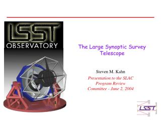
The Large Synoptic Survey Telescope Project Steven M. Kahn Friday Seminar Cornell University January 28, 2005
LSST Organization • Three main sub-project teams: Telescope/Site (NSF): NOAO, U. of Arizona Camera (DOE): SLAC, BNL, LLNL, Harvard, U. of Illinois et al. Data Management (Both): NCSA, LLNL, U. of Arizona, U. of Washington et al.
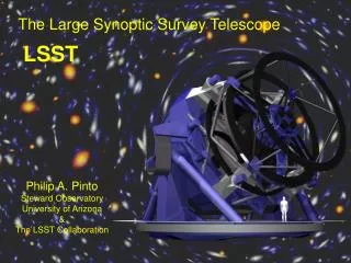
What is the LSST? • The LSST will be a large, wide-field ground-based telescope designed to provide time-lapse digital imaging of faint astronomical objects across the entire visible sky every few nights. • LSST will enable a wide variety of complementary scientific investigations, utilizing a common database. These range from searches for small bodies in the solar system to precision astrometry of the outer regions of the galaxy to systematic monitoring for transient phenomena in the optical sky. • Of particular interest for cosmology, LSST will provide strong constraints on models of dark matter and dark energy through weak lensing.
The Essence of LSST is Deep, Wide, Fast! • Dark matter/dark energy via weak lensing • Dark matter/dark energy via supernovae • Galactic Structure encompassing local group • Dense astrometry over 20,000 sq.deg: rare moving objects • Gamma Ray Bursts and transients to high redshift • Gravitational micro-lensing • Strong galaxy & cluster lensing: physics of dark matter • Multi-image lensed SN time delays: separate test of cosmology • Variable stars/galaxies: black hole accretion • QSO time delays vs z: independent test of dark energy • Optical bursters to 25 mag: the unknown • 5-band 27 mag photometric survey: unprecedented volume • Solar System Probes: Earth-crossing asteroids, Comets, TNOs
The Accelerating Universe Courtesy Supernova Cosmology Project at LBNL
Why Now? Courtesy Eric Linder
LSST and Dark Energy • LSST will measure 250,000 resolved high-redshift galaxies per square degree! The full survey will cover 18,000 square degrees. • Each galaxy will be moved on the sky and slightly distorted due to lensing by intervening dark matter. Using photometric redshifts, we can determine the shear as a function of z. • Measurements of weak lensing shear over a sufficient volume can determine DE parameters through constraints on the expansion history of the universe and the growth of structure with cosmic time.
Dealing with systematics The shear is a spin-2 field and consequently we can measure two independent ellipticity correlation functions. The lensing signal is caused by a gravitational potential and therefore should be curl-free. We can project the correlation functions into one that measures the divergence and one that measures the curl: E-B mode decomposition. E-mode (curl-free) B-mode (curl)
Results from completed surveys Since the first detections reported in spring 2000, many cosmic shear measurements have been published. Results in 2001 In general there is good agreement between surveys!
LSST and Dark Energy • The LSST Weak Lensing Survey will constrain DE via a variety of related, but different techniques: • Cluster Counts Versus Redshift: The measurement of the number density of clusters as a function of mass and redshift - dN/dMdz. • Shear Tomography: The measurement of the large-angle shear power spectrum and higher moment correlations. With photo-z’s, these can be measured as a function of cosmic time. Combining the shear power spectrum with the CMB fluctuation spectrum places constraints on w and wa. • These techniques have different dependences and different systematics. Probing the Concordance Cosmological Model in multiple ways is probably the best means we have of discovering new underlying physics.
Cluster Counting • The mass function is steep and exponentially sensitive to errors in Mlimit (z) and uncertainty in M(observables,z). • Measure mass function, determine Mlimit (z) from LSST cluster survey, devise a test that is insensitive to the limiting mass.
3D Mass Tomography From Wittman et al. 2003.
X-ray follow-up Mass X-ray Courtesy Tony Tyson and the DLS Project Team
Cluster Counting Via WL Tomograhpy • dN/dMdz constrains DE models via the dependences on the co-moving volume element, dV/dWdz, and on the exponential growth of structure, d(z). • Since WL measured DM mass directly, it does not suffer by the various forms of baryon bias and uncertainties in gas dynamical processes. • With a sky coverage of 18,000 square degrees, LSST will find 200,000 clusters. A sample this size will yield a measurement of w to 2-3%. From Haiman et al. (2005)
LSST Dark Energy Constraints from Cluster Analysis p/r= w0 + wa (1-a) a = (1+z)-1
Cosmological Constraints from Weak Lensing Shear Underlying physics is extremely simple General Relativity: FRW Universe plus the deflection formula. Any uncertainty in predictions arises from (in)ability to predict the mass distribution of the Universe Method 1:Operate on large scales in (nearly) linear regime. Predictions are as good as for CMB. Only "messy astrophysics" is to know redshift distribution of sources, which is measurable using photo-z’s. Method 2:Operate in non-linear, non-Gaussian regime. Applies to shear correlations at small angle. Predictions require N-body calculations, but to ~1% level are dark-matter dominated and hence purely gravitational and calculable with foreseeable resources. Hybrids:Combine CMB and weak lens shear vs redshift data. Cross correlations on all scales.
Measurement of the Cosmic Shear Power Spectrum • An independent probe of DE comes from the correlation in the shear in various redshift bins over wide angles. • Using photo-z’s to characterize the lensing signal improves the results dramatically over 2D projected power spectra (Hu and Keeton 2002). • A large collecting area and a survey over a very large region of sky is required to reach the necessary statistical precision. • Independent constraints come from measuring higher moment correlations, like the 3-point functions. • LSST has the appropriate etendue for such a survey. From Takada et al. (2005)
Constraints on DE Parameters From Takada et al. (2005)
LSST SNe: Std Observations • SNe from standard survey observations • ~250,000 Type Ia SNe found per year • Redshift range 0.1 < z < 0.8 • All followed with ~5 day cadence in one band (r), with 3 additional bands providing important color information for reddening, etc. • Use host photo-z’s of both the parent galaxies and the SNe themselves
w = -1.0 w = -0.9 w = -0.6 w = -0.4 z Dm = m - m(w=-0.8) 0.1 0.0 0.2 0.4 0.6 0.8 1.0 -0.1 -0.2 Equation of State Dependence Difference in apparent SN brightness vs. z WL=0.73*, flat cosmology
Standard time-domain cadence allows massively parallel SN discovery From Garnavich et al. (2005)
Crisp Images Over Entire Field L. Seppala, LLNL
Camera Challenges • Detector requirements: • 10 mm pixel size • Pixel full-well > 90,000 e– • Low noise (< 5 e– rms), fast (< 2 sec) readout ( < –30 C) • High QE 400 – 1000 nm • All of above exist, but not simultaneously in one detector • Focal plane position precision of order 3 mm • Package large number of detectors, with integrated readout electronics, with high fill factor and serviceable design • Large diameter filter coatings • Constrained volume (camera in beam) • Makes shutter, filter exchange mechanisms challenging • Constrained power dissipation to ambient • To limit thermal gradients in optical beam • Requires conductive cooling with low vibration
Science goals drive sensor requirements • High QE out to 1000nm thick silicon (> 75 µm) • PSF << 0.7” high internal field in the sensor high resistivity substrate (> 5 kohm∙cm) high applied voltages (> 50 V) • Fast f/1.2 focal ratio sensor flatness < 5µm package with piston, tip, tilt adjustable to ~1µm • Wide FOV 3200 cm2 focal plane > 200-CCD mosaic (~16 cm2 each) industrialized production process required • High throughput > 90% fill factor 4-side buttable package, sub-mm gaps • Fast readout highly-segmented sensors (~6400 output ports) > 150 I/O connections per package
Advances in State-of-the-Art needed for LSST Detector • The focal plane array will have about an order of magnitude larger number of pixels ( ~3 gigapixels) than the largest arrays realized so far. • The effective pixel readout speed will have to be about two orders of magnitude higher than in previous telescopes in order to achieve a readout time for the telescope of ~1 - 2 seconds. • The CCDs will have to have an active region ~100 µm thick to provide sufficiently high quantum efficiency at ~1000 nm, and they will have to be fully depleted (with no field free region) so that the signal charge is collected with minimum diffusion as needed to achieve a narrow point spread function. • Packaging ensuring sensor flatness and alignment in focal plane to <5µm (not achieved with presently delivered devices by industry). • Extensive use of ASICs to make the readout of a large number of output ports practical, and to reduce the number of output links and penetrations of the dewar.
LSST requires sensors in a new thickness range epi thickness limit Limit of self-supporting bulk wafers 100 LBNL technology LSST required range commercial back-thinned CCDs: Operating Voltage standard “deep depletion” 10 300 mm 200 100 0 Thickness
Importance of Depletion for PSF Diffusion:σ= d (2kT/eV)1/23.36 µm at 30 V on 100 µm, 200K (overdepleted!) E Emax=(Vdepl+Vappl)/d ~ 3 kV/cm Conductive backside window (requires special processing) Over depletion Readout electrodes Full depletion Under depletion d x 0 σdiff min≈ x = undepleted region
Strawman CCD layout under study 4k x 4k, 10 µm pixels, 32 output ports; Pixel full-well >90,000 e; Noise < 5 rms e Segmented readout to achieve the required readout time (2 seconds required, 1 second target) with moderate clock frequency (to minimize read noise and crosstalk), (e.g., 0.5 Mpixels/output read out at 250-500kHz).
Vendor guarantee Focal Plane Array Integration
FPA Structure • Modeling • Deflections, gravity • Normal modes • Thermal • x-y motions
Tiling of the Focal Plane 4° FOV 74 cm WFS 8/5/04 workshop CCDs: 3x3 3.5° FOV 64 cm X X X X X X X X X X X 4096x4096 pixels; 10 µm pixels 1678 mm2 active 41.7 mm x 41.7 mm Si 42 mm pitch (0.3 mm gaps) • 95% fill factor • 25 x 3x3 = 225 chips • If allow dummies outside 64cm, then:21 rafts with 9 live;+4 corners with 3 live ea • = 201 live chips total X X X X X X X X X X X X X wea 8/6/04
Camera Electronics Architecture • Electronics is distributed over three “thermal zones” • A front end zone, located closely behind the focal plane (analog). • A back end zone, located further away, but inside the dewar (ADC, timing and control). • External services located outside the inner dewar.
Camera Mechanical Layout 1.6m L1 L2 Shutter L3 Detector array Filter
Shutter Design One sheet design • Simplest design, fewest moving parts, fits the limited space most easily Sheet Materials • titanium or beryllium copper (good tradeoffs between modulus and yield strength)
Filter exchange mechanism 4-bar linkage allows filter to move past shutter and fit inside the outer camera Dewar
LSST Data Rates • 3.2 billion pixels read out in less than 2 sec, every 12 sec • 1 pixel = 2 Bytes (raw) • Over 3 GBytes/sec peak raw data from camera • Real-time processing and transient detection: < 10 sec • Dynamic range: 4 Bytes / pixel • > 0.6 GB/sec average in pipeline • 5000 floating point operations per pixel • 2 TFlop/s average, 9 TFlop/s peak • ~ 18 Tbytes/night