Chapter 3 Pipelining
Chapter 3 Pipelining. 3.1 Pipeline Model . Terminology task subtask stage staging register Total processing time for each task. T pl = , where t i is the processing time, d i is the delay by the staging register, and k is the number of stages.


Chapter 3 Pipelining
E N D
Presentation Transcript
3.1 Pipeline Model • Terminology • task • subtask • stage • staging register • Total processing time for each task. • Tpl = , where tiis the processing time, di is the delay by the staging register, and k is the number of stages
3.1 Pipeline Model (continued) • Total processing time for each task. • Tseq = • pipeline cycle time, tmax= Max(ti+di), 1 I k • clock frequency = 1/ tmax • pipeline cycle time tcyc can be denoted by Tseq/k + d • speedup, S = ,where N is the number of tasks.
3.1 Pipeline Model (continued) • If staging register delay is ignored and the processing times of the stages are same, tcyc = Tseq / k. Therefore, Sideal becomes • If
3.1 Pipeline Model (continued) • The total cost of the pipeline is given by C= L.k + Cp where Cp = and L is the cost of each staging register. • To minimize the composite cost per the computation rate, k =
3.1 Pipeline Model (continued) • In practice, making the delays of pipeline stages equal is a complicated and time-consuming process • It is essential to maximum performance that the stages be close to balanced. • It is done for commercial processors, although it is not easy and cheap to do • Another problem with pipelines is the overhead in term of handling exception or interrupts. • A deep pipeline increases the interrupt handling overhead.
Pipeline Types • Pipeline Types(Handler’s classification) • Instruction pipelines • FI, DI, CA, FO, EX, ST • arithmetic pipelines • processor pipelines: a cascade of processors each executing a specific module in the application program.
Instruction pipeline • reservation table • Row : stages • Column : pipeline cycles • The cycle time of instruction pipelines is often determined by the stages requiring memory access.
Control Hazard • Conditional branch instructions • The target address of branch will be known only after the evaluation of the condition. • The ways to solve control hazards • The pipeline is frozen • The pipeline predicts that the branch will not be taken. • It would be to start fetching the target instruction sequence into a buffer while the nonbranch sequence is being fed into the pipeline.
Arithmetic pipelines • Floating point addition • Consider S = A + B, where A=(Ea,Ma), B=(Eb, Mb), and S=(Es,Ms) • Addition steps (Figure 3.5) • Equalize the exponents • Add mantissas • Normalize Ms and adjust Es for the sum normalization • Round Ms • Renormalize Ms and adjust Es • Modified floating point add pipeline (Figure 3.6 & 3.7)
Arithmetic pipelines(cont.) • floating point multiplication • Consider P= A x B, where A=(Ea,Ma), B=(Eb, Mb), and P=(Ep,Mp) • Multiplication steps (Figure 3.8) • Add exponents • Multiply mantissas • Normalize Mp and adjust Ep • Round Mp • Renormalize Mp and adjust Ep • Modified floating point add pipeline (Figure 3.9)
Arithmetic pipelines(cont.) • Multifunction pipeline • To perform more than one operation • A control input is needed for proper operation of the multifunction pipeline. • Figure 3.10 : floating point add/multiplier
Classification scheme by Ramamoorthy and Li • Functionality • unifunctional • multifunctional • Configuration • static • dynamic • Mode of operation: • scalar • vector
3.2 Pipeline control and Performance • To provide the max. possible throughput, it must be kept full and flowing smoothly. • Two conditions of smooth flow of a pipeline: • the rate of input of data • data interlocks between the stages • Example 3.1 : the pipeline completes one operation per cycle(once it is full) • Example 3.2 : non-linear pipeline
Structural hazard • Due to the non-availability of appropriate hardware • One obvious way of avoiding structural hazard is to insert additional hardware into the pipeline.
Example 3.3 • Figure 3.12 depicts the operation of the pipeline • In cycle 3, 4, 5, and 6, simultaneous accesses are needed. • If we assume that the machine has separate data and instruction caches, in cycles 5 and 6 the problems are solved. • One way to solve the problem in cycle 4 is to stall the ADD instruction (Figure 3.13) • The stalling process results in a degradation of pipeline performance.
Collision vectors • Initiation : launching of an operation into the pipeline • Latency: the number of cycles that elapse between two initiation. • Latency sequence: the latencies between successive initiations • Collision: it occurs if a stage in the pipeline is required to perform more than one task at any time.
Collision vectors(cont.) • Forbidden set: the set of all possible column distances between two entries on some row of RT. • Collision vector can be derived from forbidden set F and can be utilized to control the initiation of operations in the pipelines. • CV = (vn-1,vn-2,…,v2,v1) • Vi =1 if i is in the forbidden set
Examples Example 3.4 • Overlapped RT • Collision Vector(CV) Example 3.5 & 3.6 Collision case and no collision case
Control • How to control the initiation of pipeline using CV. • Place the CV in a shift reg. • If the LSB of the shift reg. Is 1, do not initiate an operation at that cycle; shift the CV right once, inserting 0 at the vacant MSB position • If the LSB of the shift reg. Is 0, initiate a new operation at that cycle; shift the CV right once, inserting 0 at the vacant MSB position. In order to reflect the superposing status due to the new initiation over the original one, perform a bit-by-bit OR of the original CV with the content of the shift reg.
3.2.3 Performance • Figure 3.15(a) • The CV of Figure 3.11 : (00111) • Figure 3.15(a) shows the state transitions.
3.2.3 Performance • Average latency • simple cycle • greedy cycle • MAL(Minimum average Latency)
3.2.4 Multifunction Pipelines • Figure 3.17 • Vxx, Vxy, Vyx, Vyy
3.3 Other Pipeline Problems • Data Interlock: due to the sharing of resources. Data hazard • data forwarding • internal forwarding • write-read forwarding • read-read forwarding • write-write forwarding • load/store architectures versus memory/memory architectures
3.3 Other Pipeline Problems (continued) • Conditional Branches • branch prediction • delayed branch • branch-prediction buffer • branch history • multiple instruction buffers • Interrupts • precise interrupt scheme
3.4 Dynamic Pipelines • Instruction deferral • scoreboard • Tomosulo’s algorithm • Performance evaluation • maximizing the total number of initiations per unit time • minimizing the total time required to handle a specific sequences of initiation table types
3.5 Example systems • CDC Star-100 • CDC 6600 • MIPS R-4000
3.6 Summaries • Three approaches have been tried to improve the performance beyond the ideal CPI case: • superpipeline • superscalar • VLIW(Very Long Instruction Word)