Bayesian Classification
Bayesian Classification. Outline. Statistics Basics Naive Bayes Bayesian Network Applications. 有两个概率问题,都是网上玩的 8 人局情况下。 1. 我和我朋友两个人一起玩,同一势力的概率有多少? 可以分为 3 个阵营( 1 , 1 主公 +2 忠诚 2 , 4 反贼 3 ,内奸).


Bayesian Classification
E N D
Presentation Transcript
Outline • Statistics Basics • Naive Bayes • Bayesian Network • Applications
有两个概率问题,都是网上玩的8人局情况下。1.我和我朋友两个人一起玩,同一势力的概率有多少?有两个概率问题,都是网上玩的8人局情况下。1.我和我朋友两个人一起玩,同一势力的概率有多少? • 可以分为3个阵营(1,1主公+2忠诚 2,4反贼 3,内奸)
三扇门1 2 3 ,一扇门背后是巨额奖金,另外两扇的背后是“欢迎光临”。你选1号门以后,我把2号门打开,2号门显示“欢迎光临”(补充:我知道那一扇门背后有奖金的,所以绝对不开有奖金的门),然后我问你:“我现在给你多一次机会,你要坚持选你的1号门,还是转为选3 号门呢?”此为著名Monty Hall problem。
Windy=True Windy=False Play=yes Play=no Basics • Unconditional or Prior Probability • Pr(Play=yes) + Pr(Play=no)=1 • Pr(Play=yes) is sometimes written as Pr(Play) • Table has 9 yes, 5 no • Pr(Play=yes)=9/(9+5)=9/14 • Thus, Pr(Play=no)=5/14 • Joint Probability of Play and Windy: • Pr(Play=x,Windy=y) for all values x and y, should be 1 3/14 6/14 3/14 ?
Probability Basics • Conditional Probability • Pr(A|B) • # (Windy=False)=8 • Within the 8, • #(Play=yes)=6 • Pr(Play=yes | Windy=False) =6/8 • Pr(Windy=False)=8/14 • Pr(Play=Yes)=9/14 • Applying Bayes Rule • Pr(B|A) = Pr(A|B)Pr(B) / Pr(A) • Pr(Windy=False|Play=yes)= 6/8*8/14/(9/14)=6/9
Conditional Independence • “A and P are independent given C” • Pr(A | P,C) = Pr(A | C) C A P Probability F F F 0.534 F F T 0.356 F T F 0.006 F T T 0.004 T F F 0.048 T F T 0.012 T T F 0.032 T T T 0.008 Ache Cavity Probe Catches
C A P Probability F F F 0.534 F F T 0.356 F T F 0.006 F T T 0.004 T F F 0.012 T F T 0.048 T T F 0.008 T T T 0.032 Suppose C=True Pr(A|P,C) = 0.032/(0.032+0.048) = 0.032/0.080 = 0.4 Pr(A|C) = 0.032+0.008/ (0.048+0.012+0.032+0.008) = 0.04 / 0.1 = 0.4 Conditional Independence • “A and P are independent given C” • Pr(A | P,C) = Pr(A | C) and also Pr(P | A,C) = Pr(P | C)
Outline • Statistics Basics • Naive Bayes • Bayesian Network • Applications
Naïve Bayesian Models • Two assumptions: Attributes are • equally important • statistically independent (given the class value) • This means that knowledge about the value of a particular attribute doesn’t tell us anything about the value of another attribute (if the class is known) • Although based on assumptions that are almost never correct, this scheme works well in practice!
Why Naïve? • Assume the attributes are independent, given class • What does that mean? play outlook temp humidity windy Pr(outlook=sunny | windy=true, play=yes)= Pr(outlook=sunny|play=yes)
Is the assumption satisfied? • #yes=9 • #sunny=2 • #windy, yes=3 • #sunny|windy, yes=1 Pr(outlook=sunny|windy=true, play=yes)=1/3 Pr(outlook=sunny|play=yes)=2/9 Pr(windy|outlook=sunny,play=yes)=1/2 Pr(windy|play=yes)=3/9 Thus, the assumption is NOT satisfied. But, we can tolerate some errors (see later slides)
Probabilities for the weather data • A new day:
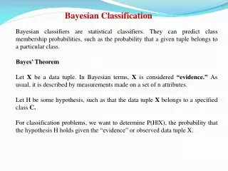
Bayes’ rule • Probability of event H given evidence E: • A priori probability of H: • Probability of event before evidence has been seen • A posteriori probability of H: • Probability of event after evidence has been seen
Naïve Bayes for classification • Classification learning: what’s the probability of the class given an instance? • Evidence E = an instance • Event H = class value for instance (Play=yes, Play=no) • Naïve Bayes Assumption: evidence can be split into independent parts (i.e. attributes of instance are independent)
The weather data example Evidence E Probability for class “yes”
The “zero-frequency problem” • What if an attribute value doesn’t occur with every class value (e.g. “Humidity = high” for class “yes”)? • Probability will be zero! • A posteriori probability will also be zero! (No matter how likely the other values are!) • Remedy: add 1 to the count for every attribute value-class combination (Laplace estimator) • Result: probabilities will never be zero! (also: stabilizes probability estimates)
Modified probability estimates • In some cases adding a constant different from 1 might be more appropriate • Example: attribute outlook for class yes • Weights don’t need to be equal (if they sum to 1) Sunny Overcast Rainy
Missing values • Training: instance is not included in frequency count for attribute value-class combination • Classification: attribute will be omitted from calculation • Example:
Dealing with numeric attributes • Usual assumption: attributes have a normal or Gaussian probability distribution (given the class) • The probability density function for the normal distribution is defined by two parameters: • The sample mean : • The standard deviation : • The density function f(x):
Statistics for the weather data • Example density value:
Classifying a new day • A new day: • Missing values during training: not included in calculation of mean and standard deviation
Probability densities • Relationship between probability and density: • But: this doesn’t change calculation of a posteriori probabilities because cancels out • Exact relationship:
Example of Naïve Bayes in Weka • Use Weka Naïve Bayes Module to classify • Weather.nominal.arff
Discussion of Naïve Bayes • Naïve Bayes works surprisingly well (even if independence assumption is clearly violated) • Why? Because classification doesn’t require accurate probability estimates as long as maximum probability is assigned to correct class • However: adding too many redundant attributes will cause problems (e.g. identical attributes) • Note also: many numeric attributes are not normally distributed
Outline • Statistics Basics • Naive Bayes • Bayesian Network • Applications
C P(A) T 0.4 F 0.02 P(C) .1 C P(P) T 0.8 F 0.4 Conditional Independence Conditional probability table (CPT) • Can encode joint probability distribution in compact form C A P Probability F F F 0.534 F F T 0.356 F T F 0.006 F T T 0.004 T F F 0.012 T F T 0.048 T T F 0.008 T T T 0.032 Ache Cavity Probe Catches
Creating a Network • 1: Bayes net = representation of a JPD • 2: Bayes net = set of cond. independence statements • If create correct structure that represents causality • Then get a good network • i.e. one that’s small = easy to compute with • One that is easy to fill in numbers
Example • My house alarm system just sounded (A). • Both an earthquake (E) and a burglary (B) could set it off. • John will probably hear the alarm; if so he’ll call (J). • But sometimes John calls even when the alarm is silent • Mary might hear the alarm and call too (M), but not as reliably • We could be assured a complete and consistent model by fully specifying the joint distribution: • Pr(A, E, B, J, M) • Pr(A, E, B, J, ~M) • etc.
Structural Models Instead of starting with numbers, we will start with structural relationships among the variables There is a direct causal relationship from Earthquake to Alarm There is a direct causal relationship from Burglar to Alarm There is a direct causal relationship from Alarm to JohnCall Earthquake and Burglar tend to occur independently etc.
Earthquake Burglary Alarm MaryCalls JohnCalls Possible Bayesian Network
P(E) .002 P(B) .001 B T T F F E T F T F P(A) .95 .94 .29 .01 A T F P(J) .90 .05 A T F P(M) .70 .01 Complete Bayesian Network Earthquake Burglary Alarm MaryCalls JohnCalls
Microsoft Bayesian Belief Net • http://research.microsoft.com/adapt/MSBNx/ • Can be used to construct and reason with Bayesian Networks • Consider the example
Mining for Structural Models • Difficult to mine • Some methods are proposed • Up to now, no good results yet • Often requires domain expert’s knowledge • Once set up, a Bayesian Network can be used to provide probabilistic queries • Microsoft Bayesian Network Software
Use the Bayesian Net for Prediction • From a new day’s data we wish to predict the decision • New data: X • Class label: C • To predict the class of X, is the same as asking • Value of Pr(C|X)? • Pr(C=yes|X) • Pr(C=no|X) • Compare the two
Outline • Statistics Basics • Naive Bayes • Bayesian Network • Applications
Applications of Bayesian Method • Gene Analysis • Nir Friedman Iftach Nachman Dana Pe’er, Institute of Computer Science, Hebrew University • Text and Email analysis • Spam Email Filter • Microsoft Work • News classification for personal news delivery on the Web • User Profiles • Credit Analysis in Financial Industry • Analyze the probability of payment for a loan
Gene Interaction Analysis • DNA • Gene • DNA is a double-stranded molecule • Hereditary information is encoded • Complementation rules • Gene is a segment of DNA • Contain the information required to make a protein
Gene Interaction Result: • Example of interaction between proteins for gene SVS1. • The width of edges corresponds to the conditional probability.