Scheduling for Multithreaded Chip Multiprocessors (Multithreaded CMPs)
Scheduling for Multithreaded Chip Multiprocessors (Multithreaded CMPs). CMTs (Chip multithreaded processors). CMP plus hardware multithreading Supports a large number of thread contexts Can hide memory latency by spawning multiple threads High contention for shared resources

Scheduling for Multithreaded Chip Multiprocessors (Multithreaded CMPs)
E N D
Presentation Transcript
Scheduling for Multithreaded Chip Multiprocessors (Multithreaded CMPs)
CMTs (Chip multithreaded processors) • CMP plus hardware multithreading • Supports a large number of thread contexts • Can hide memory latency by spawning multiple threads • High contention for shared resources • Commercial Processors • Intel Core 2 Duo: I Core 2 Duo: 2 cores, ... x2 L1 Cache, 4MB L2 Cache,1.86–2.93 Ghz • AMD Athlon 64 X2: 2 cores, 128KB x2 L1 Cache, 2MB L2 Cache,2.00–2.60 Ghz • SUN UltraSPARC T1 (Niagara): up to 8 cores, 24KB x8 L1 Cache, 3MB L2 Cache, 1.00–1.20Ghz
Multithreading Approaches • Coarse grained • Context switch on memory access (switch on cache miss) • High switch cost (decision made late in the pipeline) • Fine grained • Switches threads on every cycle • Performance of a single thread is very poor • Preferred by CMT processors
Pipeline usage and Scheduling • Thread Classification (can be done on CPI) • Compute Intensive • Functional unit utilization is high • Memory Intensive • Threads frequently stall for memory access • OS Schedule has to balance demand for pipeline resources across cores by co-scheduling memory intensive and compute intensive applications
Pipeline Contention Study (1) • Experiment performed using modified SIMICS (SAM simulator) • 4 cores and 4 thread contexts for each core • Tried several ways to schedule 16 threads • (a) and (b) match compute–intensive threads with memory–intensive threads. , (c) and (d) place compute–intensive threads on the same core.
Pipeline contention Study (2) • Results as expected • Schedules (a) and (b) outperform (c) and (d) • However, • Threads required large CPI variation not always possible (Apps are very rarely just compute or memory intensive, they are often a mixture of both) • For real benchmarks, performance gains are modest (e.g. 5% improvement for SPEC)
L1 Data Cache Contention • Each core has four threads executing the same benchmark • 32KB caches seem sufficient for the benchmarks studied • IPC not sensitive to L1 miss ratio
L2 Cache Contention • 2 Core , 4 thread contexts per core, 9 benchmarks, two copies (18 benchmarks), 8 KB L1 • L2 expected to have greater impact due to miss resulting in high latency memory access • Results corroborate L2 impact • IPC very sensitive to L2 miss ratio • Summary: Equip the OS to handle L2 cache shortage
Balance-Set Scheduling • Originally proposed as a technique for virtual memory by Denning • Concept: working set • Each program has a footprint, which if cached can decrease execution time • Solution: Schedule threads such that the combined working sets fit in the cache • Problem: Working sets are not very good indicators of cache behavior • Programs do not access working sets uniformly
The Reuse-Distance Model • Proposed by Berg and Hagersten • Reuse-Distance: Time b/w successive refs to the same memory location (measured in num. of memory refs) • Tries to capture temporal locality lower the reuse-distance, greater the chance of reuse • Reuse-Distance histogram can be built at runtime • Parallels to LRU stack used in LRU replacement
Two Methods • COMB: (i) sum the number of references for each reuse distance in each histogram, (ii) and multiply each reuse distance by the number of threads in the group, (iii) apply the reuse–distance estimation on the resulting histogram AVG: (i) assume that each thread runs with its own dedicated partition of a cache, (ii) estimate ratios for individual threads, (iii) compute the average.
Comparison of COMB Vs AVG • Both COMB and AVG come within 17% of actual • COMB is computationally expensive • In a machine with 32 thread contexts and 100 threads the scheduler has to combine 100C32 histograms • AVG wins!
The Scheduling Algorithm (1) • Step 1: Computing miss rate estimations (Periodically) • With N runnable threads and M hardware contexts, compute the miss rate estimations of the NCM groups of M threads by using the reuse–distance model and AVG • Step 2: Choosing the L2 miss ratio threshold (Periodically) • Picks the smallest miss ratio among threads containing the greediest (cache intensive) thread • Step 3: Identify the groups that will produce low cache miss ratios (Periodically) • The groups below the threshold are candidate groups (Every runnable thread has to be in a candidate group) • Step 4: Scheduling decision (Every time a time slice expires) • Choose a group from the set of candidate groups and schedule the threads in the group to run during the current time slice
The Scheduling Algorithm (2) • To choose thread groups there can be two policies: performance–oriented (PERF) and fairness–oriented (FAIR) • PERF: we select the group with the lowest miss ratio and containing threads that have not yet been selected, until each thread is represented in the schedule • With FAIR, we select the group with the greatest number of the least frequently selected threads
Performance Evaluation • The 18–thread SPEC workload setup reused • Reuse-distance histograms computed offline • All combinations examined for computing candidate set • Default refers to the SOLARIS default scheduler • 19-37% improvement using PERF (9-18% using FAIR) • Doubling L2 gives same benefits as using PERF
References • "Chip Multithreading Systems Need a New Operating System Scheduler", Alexandra Fedorova, Christopher Small, Daniel Nussbaum, and Margo Seltzer • "Performance of Multithreaded Chip Multiprocessors and Implications for Operating System Design", A. Fedorova, M. Seltzer, C. Small, and D. Nussbaum