Download
1 / 25
260 likes | 670 Vues
Budget Constraints. ECO61 Udayan Roy Fall 2008. Prices, quantities, and expenditures. P X is the price of good X It is measured in dollars per unit of good X The consumer pays this price no matter what quantity she buys.

E N D
Budget Constraints ECO61 Udayan Roy Fall 2008
Prices, quantities, and expenditures • PX is the price of good X • It is measured in dollars per unit of good X • The consumer pays this price no matter what quantity she buys. • That is, there are no quantity discounts and there is no rationing • X is also the quantity of good X that is purchased by the consumer • It is measured in units of good X per unit of time • PX X = PXX is the consumer’s expenditure on good X
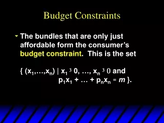
Budget constraint • Assume a world with only two consumer goods, X and Y • Total expenditure = PXX + PYY • M is the consumer’s income or budget • The consumer cannot spend more than her budget allows • PXX + PYY ≤ M is the consumer’s budget constraint
“More-is-better” implies budget exhaustion • A rational consumer will spend every penny available. • PXX + PYY ≤M becomes PXX + PYY =M • Here’s an example:
Saving • The budget constraint PXX + PYY = M does not imply that saving is being ignored. • We saw earlier that, to an economist, “food delivered now” and “food delivered in the future” are different goods • The former could be our good X and the latter could be good Y • Then PYY would represent saving for the future.
Saving • You may pay today for something that will be delivered at some date in the future. • For example, you may pay Long Island University today for courses you plan to take in 2015 • You may pay today to reserve hotel rooms in London for the 2012 Olympics • You may pay today for the future delivery of the National Geographic magazine • These purchases are the same as saving for the future.
Budget constraint algebra • If X = 0, then Y = M/PY • This is the maximum amount of good Y that the consumer can buy • Similarly, the maximum amount of good X that the consumer can buy is M/PX • If the consumer’s income (M) increases, both maximums will increase by the same proportion
Budget Constraint: Graph • PSS + PBB = M is the budget constraint • It can be graphed into the budget line:
Budget constraint algebra • If X increases by one unit, then Y must decrease by PX/PY units • This is at the heart of the consumer’s tradeoff • PX/PY is also called the relative price of good X (in units of good Y)
Budget Constraint • Consider Lisa, who buys only burritos (B) and pizza (Z) • If pZ= $1, pB= $2, and M= $50, then:
Possible Allocations of Lisa’s Budget Between Burritos and Pizza Lisa’s budget is $50. Burritos are $2 each and pizzas are $1 each.
Budget Constraint: graph • From previous slide we have that if: • pZ= $1, pB= $2, and M= $50, then the budget constraint, L1, is: Amount of Burritos consumed if all income is allocated for Burritos. a = 25 M / p B itos per semester b 20 1 L r Amount of Pizza consumed if all income is allocated for Pizza. , Bur c B 10 Opportunity set d = 50 M p 0 10 30 / Z Z , Pizzas per semester
The Slope of the Budget Constraint • We have seen that the budget constraint for Lisa is given by the following equation: • The slope of the budget line is the rate at which Lisa can trade burritos for pizza in the marketplace Slope = DB/DZ
Changes in the Budget Constraint: An increase in the Price of Pizzas. PZ = $1 $2 M - B = Z Slope = -$1/$2 = -0.5 PB PB If the price of Pizza doubles, (increases from $1 to $2) the slope of the budget line increases 25 itos per semester p = $1 Z r , Bur B Loss This area represents the bundles she can no longer afford pZ = $2 0 25 50 Slope = -$2/$2 = -1 Z , Pizzas per semester
How taxes affect the budget constraint • A tax of TZ dollars per pizza has the effect of raising the price paid by the buyer from PZ to PZ + TZ. • Therefore, the effect is essentially the same as in the previous slide
Changes in the Budget Constraint: Increase in Income (M) PZ $100 $50 - Z B = PB PB If Lisa’s income increases by $50 the budget line shifts to the right (with the same slope!) 50 = M $100 B, Burritos per semester 25 This area represents the new consumption bundles she can now afford Gain = M $50 0 50 100 Z , Pizzas per semester
Solved Problem • A government rations water, setting a quota on how much a consumer can purchase. • If a consumer can afford to buy 12 thousand gallons a month but the government restricts purchases to no more than 10 thousand gallons a month, how does the consumer’s opportunity set change?
Income in the budget constraint • We have seen that the consumer’s budget is affected by her income (M) • Therefore, the consumer’s choices (of X and Y) are affected by her income • But it has been implied that income (M) is not affected by the consumer’s choices (of X and Y) • This is not always true: the consumer’s choices (of X and Y) may affect her income (M)
Income in the budget constraint • It is also implicit in my discussion of the budget constraint that income (M) is not affected by prices (of X and Y) • This is not always true: theprices of goods (PX and PY) may affect income (M)
Leisure and consumption (24w + M*)/PY • The price of leisure (N) is the wage (w) that is lost y Time const r aint a , Goods per d Slope = -w/PY When w/PY decreases, the budget constraint rotates down Y Consumption with non-labor income (M*/PY) 0 N N 24 N , Leisure hours per d a y 1 2 24 H H 0 H , W o r k hours per d a y 1 2
Leisure and consumption II: M* = 0 24w/PY • The price of leisure (N) is the wage (w) that is lost y a , Goods per d Y Slope = -w/PY When w/PY decreases, the budget constraint rotates down 24w/w = 24 0 N N 24 N , Leisure hours per d a y 1 2 24 H H 0 H , W o r k hours per d a y 1 2
Progressive income tax • Now we have a 20% income tax, but only on income in excess of Y0. y 24w (1-0.20)/PY a , Goods per d Slope = -w (1-0.20)/PY Y Y0 Slope = -w/PY 24w/w = 24 0 N N 24 N , Leisure hours per d a y 1 2 24 H H 0 H , W o r k hours per d a y 1 2
Income is affected by choices • Other examples where consumers’ choices affect their incomes • How much we save today will affect our future interest income • How much we spend today on which asset (stocks, bonds, college courses) will affect our future incomes