Section 9.4
Section 9.4. How Can We Analyze Dependent Samples?. Dependent Samples. Each observation in one sample has a matched observation in the other sample The observations are called matched pairs. Example: Matched Pairs Design for Cell Phones and Driving Study.

Section 9.4
E N D
Presentation Transcript
Section 9.4 How Can We Analyze Dependent Samples?
Dependent Samples • Each observation in one sample has a matched observation in the other sample • The observations are called matched pairs
Example: Matched Pairs Design for Cell Phones and Driving Study • The cell phone analysis presented earlier in this text used independent samples: • One group used cell phones • A separate control group did not use cell phones
Example: Matched Pairs Design for Cell Phones and Driving Study • An alternative design used the same subjects for both groups • Reaction times are measured when subjects performed the driving task without using cell phones and then again while using cell phones
Example: Matched Pairs Design for Cell Phones and Driving Study Data:
Example: Matched Pairs Design for Cell Phones and Driving Study • Benefits of using dependent samples (matched pairs): • Many sources of potential bias are controlled so we can make a more accurate comparison • Using matched pairs keeps many other factors fixed that could affect the analysis • Often this results in the benefit of smaller standard errors
Example: Matched Pairs Design for Cell Phones and Driving Study • To Compare Means with Matched Pairs, Use Paired Differences: • For each matched pair, construct a difference score • d = (reaction time using cell phone) – (reaction time without cell phone) • Calculate the sample mean of these differences: xd
For Dependent Samples (Matched Pairs) Mean of Differences = Difference of Means
For Dependent Samples (Matched Pairs) • The difference (x1 – x2) between the means of the two samples equals the mean xd of the difference scores for the matched pairs • The difference (µ1 – µ2) between the population means is identical to the parameter µd that is the population mean of the difference scores
For Dependent Samples (Matched Pairs) • Let n denote the number of observations in each sample • This equals the number of difference scores • The 95 % CI for the population mean difference is:
For Dependent Samples (Matched Pairs) • To test the hypothesis H0: µ1 = µ2 of equal means, we can conduct the single-sample test of H0: µd = 0 with the difference scores • The test statistic is:
For Dependent Samples (Matched Pairs) • These paired-difference inferences are special cases of single-sample inferences about a population mean so they make the same assumptions
Paired-difference Inferences • Assumptions: • The sample of difference scores is a random sample from a population of such difference scores • The difference scores have a population distribution that is approximately normal • This is mainly important for small samples (less than about 30) and for one-sided inferences
Paired-difference Inferences • Confidence intervals and two-sided tests are robust: They work quite well even if the normality assumption is violated • One-sided tests do not work well when the sample size is small and the distribution of differences is highly skewed
Example: Matched Pairs Analysis for Cell Phones and Driving Study • Boxplot of the 32 difference scores
Example: Matched Pairs Analysis for Cell Phones and Driving Study • The box plot shows skew to the right for the difference scores • Two-sided inference is robust to violations of the assumption of normality • The box plot does not show any severe outliers
Example: Matched Pairs Analysis for Cell Phones and Driving Study
Example: Matched Pairs Analysis for Cell Phones and Driving Study • Significance test: • H0: µd = 0 (and hence equal population means for the two conditions) • Ha: µd ≠ 0 • Test statistic:
Example: Matched Pairs Analysis for Cell Phones and Driving Study • The P-value displayed in the output is 0.000 • There is extremely strong evidence that the population mean reaction times are different
Example: Matched Pairs Analysis for Cell Phones and Driving Study • 95% CI for µd =(µ1 - µ2):
Example: Matched Pairs Analysis for Cell Phones and Driving Study • We infer that the population mean when using cell phones is between about 32 and 70 milliseconds higher than when not using cell phones • The confidence interval is more informative than the significance test, since it predicts just how large the difference must be
Section 9.5 How Can We Adjust for Effects of Other Variables?
A Practically Significant Difference • When we find a practically significant difference between two groups, can we identify a reason for the difference? • Warning: An association may be due to a lurking variable not measured in the study
Example: Is TV Watching Associated with Aggressive Behavior? • In a previous example, we saw that teenagers who watch more TV have a tendency later in life to commit more aggressive acts • Could there be a lurking variable that influences this association?
Control Variable • A control variable is a variable that is held constant in a multivariate analysis (more than two variables)
Can An Association Be Explained by a Third Variable? • Treat the third variable as a control variable • Conduct the ordinary bivariate analysis while holding that control variable constant at fixed values • Whatever association occurs cannot be due to effect of the control variable