Download

1 / 89
890 likes | 1.03k Vues
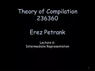
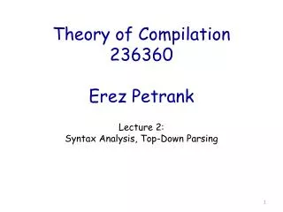
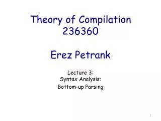
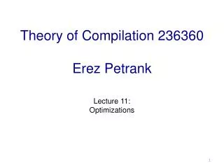
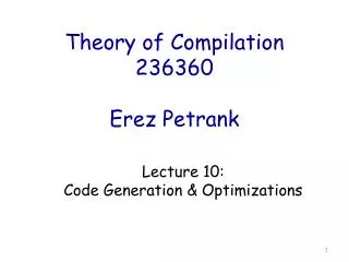
Theory of Compilation 236360 Erez Petrank. Lecture 3 : Syntax Analysis: Bottom-up Parsing. Source text. txt. Executable code. exe. You are here. Compiler. Lexical Analysis. Syntax Analysis Parsing. Semantic Analysis. Inter. Rep. (IR). Code Gen. Parsers: from tokens to AST.

E N D
Theory of Compilation 236360ErezPetrank Lecture 3: Syntax Analysis: Bottom-up Parsing
Source text txt Executable code exe You are here Compiler LexicalAnalysis Syntax Analysis Parsing SemanticAnalysis Inter.Rep. (IR) Code Gen.
Parsers: from tokens to AST <ID,”b”> <MULT> <ID,”b”> <MINUS> <INT,4> <MULT> <ID,”a”> <MULT> <ID,”c”> expression SyntaxTree expression term MINUS expression MULT factor term term ID term MULT factor term MULT factor ‘c’ factor ID ID factor ID ‘b’ ID ‘a’ ‘b’ ‘4’ LexicalAnalysis Syntax Analysis Sem.Analysis Inter.Rep. Code Gen.
Parsing • A context free language can be recognized by a non-deterministic pushdown automaton. • It can be recognized in exponential time via backtracking, • And using dynamic programming in O(n3). • We want efficient parsers • Linear in input size • We sacrifice generality for efficiency
Reminder: Efficient Parsers • Top-down (predictive parsing) already read… to be read… • Bottom-up (shift reduce)
LR(k) Grammars • A grammar is in the class LR(K) when it can be derived via: • Bottom-up derivation • Scanning the input from left to right (L) • Producing the rightmost derivation (R) • With lookahead of k tokens (k) • A language is said to be LR(k) if it has an LR(k) grammar • The simplest case is LR(0), which we discuss next.
LR is More Powerful, But… • Any LL(k) language is also in LR(k) (and not vice versa), i.e., LL(k) ⊂ LR(k). • But the lookahead is counted differently in the two cases. • In an LL(k) derivation the algorithm sees k tokens of the right-hand side of the rule and then must select the derivation rule. • With LR(k), the algorithm sees all right-hand side of the derivation rule plus k more tokens. • LR(0) sees the entire right-side. • LR is more popular today. • We will see Yacc, a parser generator for LR parsing, in the exercises and homework.
An Example: a Simple Grammar E → E * B | E + B | B B → 0 | 1 • Let us number the rules: (1) E → E * B (2) E → E + B (3) E → B (4) B → 0 (5) B → 1
Goal: Reduce the Input to the Start Symbol Example: 0 + 0 * 1 B + 0 * 1 E + 0 * 1 E + B * 1 E * 1 E * B E E E → E * B | E + B | B B → 0 | 1 * E B 1 + E B B 0 0 Go over the input so far, and upon seeing a right-hand side of a rule, “invoke” the rule and replace the right-hand side with the left-hand side (which is a single non-terminal)
Use Shift & Reduce E → E * B | E + B | B B → 0 | 1 In each stage, we shift a symbol from the input to the stack, or reduce according to one of the rules. Example: “0+0*1”. Stack Input action 0+0*1$ shift 0 +0*1$ reduce B +0*1$ reduce E +0*1$ shift E+ 0*1$ shift E+0 *1$ reduce E+B *1$ reduce E *1$ shift E* 1$ shift E*1 $ reduce E*B $ reduce E $ accept E * E B 1 + E B B 0 0
How does the parser know what to do? • A state will keep the info gathered so far. • A table will tell it “what to do” based on current state and next token. • Some info will be kept in a stack.
LR(0) Parsing Input Action Table Parser Stack Goto table Output
States and LR(0) Items E → E * B | E + B | B B → 0 | 1 • The state will “remember” the potential derivation rules given the part that was already identified. • For example, if we have already identified E then the state will remember the two alternatives: (1) E →E * B, (2) E → E + B • Actually, we will also remember where we are in each of them: (1) E →E ●* B, (2) E → E ● + B • A derivation rule with a location marker is called LR(0) item. • The state is actually a set of LR(0) items. E.g., q13= { E → E ● * B , E → E ● + B}
Intuition • We gather the input token by token until we find a right-hand side of a rule and then we replace it with the variable on the left side. • Going over a token and remembering it in the stack is a shift. • Each shift moves to a state that remembers what we’ve seen so far. • A reduce replaces a string in the stack with the variable that derives it.
Why do we need a stack? • Suppose so far we have discovered E → B →0 and gather information on “E +”. • In the given grammar this can only mean E → E +● B • Suppose state q6 represents this possibility. • Now, the next token is 0, and we need to ignore q6 for a minute, and work on B → 0 to obtain E+B. • Therefore, we push q6 to the stack, and after identifying B, we pop it to continue. E + E B 0 B 0 0 (q4,E) (q6,+) (q1,0) top
The Stack • The stack contains states. • For readability we will also include variables and tokens. (The algorithm does not need it.) • Except for the q0 in the bottom of the stack, the rest of the stack will contains pairs of (state, token) or (state, variable). • The initial stack contains the initial variable only. • At each stage we need to decide if to shift the next token to the stack (and change to the appropriate state) or apply a “reduce”. • The action table tells us what to do based on current state and next token: s n : shift and move to qn. r m: reduce according to production rule m. (also accept and error).
The Goto Table • The second table serves reduces. • After reducing a right-hand side to the deriving variable, we need to decide what the next state is. • This is determined by the previous state (which is on the stack) and the variable we got. • Suppose we reduce according to M →β. • We remove β from the stack, and look at the state q that is currently at the top. GOTO(q,M) specifies the next state.
For example… (1) E → E * B (2) E → E + B (3) E → B (4) B → 0 (5) B → 1
(1) E → E * B (2) E → E + B (3) E → B (4) B → 0 (5) B → 1 An Execution Example: 0 + 0 * 1 q1 0 q0 q0
(1) E → E * B (2) E → E + B (3) E → B (4) B → 0 (5) B → 1 An Execution Example: 0 + 0 * 1 q6 + ● ● ● q1 q4 q3 q3 0 B E E q0 q0 q0 q0 q0
The Algorithm Formally • Initiate the stack to q0. • Repeat until halting: • Consider action [t,q] for q at the head of the stack and t the next token. • “Shift n”: remove t from the input and push t and then qn to the stack. • “Reduce m”, where Rule m is: M →β: • Remove |β| pairs from the stack, let q be the state at the top of the stack. • Push M and the state Goto[q,M] to the stack. • “accept”: halt successfully. • Empty cell: halt with an error.
LR(0) Item To be matched Already matched Input E ➞ 𝛂β So far we’ve matched α, expecting to see β
LR(0) Items N αβ Shift Item N αβ Reduce Item
Using LR Items to Build the Tables • Typically a state consists of several LR items. • For example, if we identified a string that is reduced to E, then we may be in one of the following LR items: E → E ● + B or E → E ● *B • Therefore one of the states will be:q = {E → E ● + B , E → E ● * B}. • But if the current state includes E → E + ●B, then we must be able to let B be derived: Closure!
Adding the Closure • If the current state has the item E → E + ● B, then it should be possible to add derivation of B, e.g., to 0 or 1. • Generally, if a state includes an item in which the dot stands before a non-terminal, then we add all the rules for this non-terminal with a dot in the beginning. • Definition: the closure set for a set of items is the set of items in which for every item in the set of the form A → 𝛂 ● B β, the set contains an item B → ● δ, for each rule of the form B → δin the grammar. • Building the closure set is iterative, as δ may also begin with a variable.
Closure: an Example • For example, consider the grammar:and the set: C = { E → E + ●B } • C’s closure is: clos(C) = { E → E + ●B , B → ●0 , B → ●1 } • And this will be the state that will be used for the parser. E → E * B | E + B | B B → 0 | 1
Extended Grammar • Goal: easy termination. • We will assume that the initial variable only appears in a single rule. This guarantee that the last reduction can be (easily) determined. • A grammar can be (easily) extended to have such structure. Example: the grammar (1) E → E * B (2) E → E + B (3) E → B (4) B → 0 (5) B → 1 • Can be extended into : • (0) S → E • (1) E → E * B • (2) E → E + B • (3) E → B • (4)B → 0 • (5)B → 1
The Initial State • To build the action/goto table, we go through all possible states possible during derivation. • Each state represents a (closure) set of LR(0) items. • The initial state q0 is the closure of the initial rule. • In our example the initial rule is S → ● E, and therefore the initial state is q0 = clos({S → ● E }) = {S → ● E , E → ● E * B , E → ● E + B , E → ● B , B → ● 0 , B → ● 1} We go on and build all possible continuations by seeing a single token (or variable).
The Next States • For each possible terminal or variable x, and each possible state (closure set) q, • Find all items in the set of q in which the dot is before an x. We denote this set by q|x • Move the dot ahead of the x in all items in q|x. • Find the closure of the obtained set: this is the state into which we move from q upon seeing x. • Formally, the next set from a set S and the next symbol X • step(S,X) = { N➞αXβ | N➞αXβ in the item set S} • nextSet(S,X) = -closure(step(S,X))
The Next States • Recall that in our example: q0 = clos({S → ● E }) = {S → ● E , E → ● E * B , E → ● E + B , E → ● B , B → ● 0 , B → ● 1} Let us check which states are reachable from it.
States reachable from q0 in the example: State q1: x = 0 q0|0= { B →● 0 } q1= clos(q0|0) = { B → 0● } State q2: x = 1 q0|1= { B → ● 1 } q2= clos({ B → 1 ● }) = { B → 1 ∙ } State q4: x = B q0|B = { E → ∙ B } q4 = clos ({ E → B ∙ }) = {E →B∙} State q3: x = E q0|E= {S → ∙ E , E → ∙ E * B , E → ∙ E + B} q3 = clos ({S → E ∙ , E → E ∙ * B , E → E ∙ + B}) ={S → E∙, E → E∙*B , E → E ∙ + B}
From these new states there are more reachable states • From q1, q2, q4, there are no continuations because the dot is in the end of any item in their sets. • From state q3 we can reach the following two states: מצב 5q: x = * q3|* = { E → E ∙ * B } q5= clos ({ E → E * ∙ B }) = { E → E * ∙ B , B → ∙ 0 , B → ∙ 1 } מצב 6q: q6= { E → E + ∙ B , B → ∙ 0 , B → ∙ 1 }
Finally, • From q5 we can proceed with x=0, or x=1, or x=B. • But for x=0 we reach q1 again and for x=1 we reach q2. • For x=B we get q7: • Similarly, from q6 with x=B we get q8: • These two states have no continuations. (Why?) State q7: clos(q7) = { E → E * B ∙ } State q8: clos(q8) = { E → E + B ∙ }
Building the Tables • A row for each state. • If qj was obtained when x comes after qi, then in row qi and column x, we write j.
Building the tables: accept • Add “acc” in column $ for each state that has S → E ● as an item.
Building the Tables: Shift • Any number n in the action table becomes s n.
Building the Tables: Reduce • For any state whose set includes the item A → α●, such that A → α is production rule m (m>o) : • Fill all columns of that state in the action table with “r m”.
Note LR(0) • When a reduce is possible, we execute it without checking the next token.
Another Example Z ➞ exprEOF expr ➞ term | expr+ term term ➞ ID | (expr) Z ➞ E $ E ➞ T | E + T T ➞ i | ( E ) (just shorthand of the grammar on the top)
Example: Parsing with LR Items Z ➞ E $ E ➞ T | E + T T ➞ i | ( E ) Input: i + i $ } Z ➞ E $ E ➞ T E ➞ E + T Closure T ➞ i T ➞ (E )
Input: i + i $ Shift Z ➞ E $ E ➞ T | E + T T ➞ i | ( E ) i Z ➞ E $ T ➞ i Reduce item! E ➞ T E ➞ E + T T ➞ i T ➞ (E )
Input: i + i $ Z ➞ E $ E ➞ T | E + T T ➞ i | ( E ) T i Z ➞ E $ Reduce item! E ➞ T E ➞ T E ➞ E + T T ➞ i T ➞ (E )
Input: i + i $ Z ➞ E $ E ➞ T | E + T T ➞ i | ( E ) E T i Z ➞ E $ Reduce item! E ➞ T E ➞ T E ➞ E + T T ➞ i T ➞ (E )
Input: i + i $ Z ➞ E $ E ➞ T | E + T T ➞ i | ( E ) E + T i Z ➞ E $ Z ➞ E$ E ➞ T E ➞ E + T E ➞ E+T T ➞ i T ➞ (E )
Input: i + i $ Z ➞ E $ E ➞ T | E + T T ➞ i | ( E ) E + i T i Z ➞ E $ Z ➞ E$ E ➞ E+T E ➞ T T ➞ i E ➞ E + T E ➞ E+T T ➞ (E ) T ➞ i T ➞ (E )
Input: i + i $ Z ➞ E $ E ➞ T | E + T T ➞ i | ( E ) E + i $ T i Reduce item! Z ➞ E $ Z ➞ E$ E ➞ E+T E ➞ T T ➞ i T ➞ i E ➞ E + T E ➞ E+T T ➞ (E ) T ➞ i T ➞ (E )
Input: i + i $ Z ➞ E $ E ➞ T | E + T T ➞ i | ( E ) E + T T i i Z ➞ E $ Z ➞ E$ E ➞ E+T E ➞ T T ➞ i E ➞ E + T E ➞ E+T T ➞ (E ) T ➞ i T ➞ (E )
Input: i + i $ Z ➞ E $ E ➞ T | E + T T ➞ i | ( E ) E + T $ T i i Reduce item! Z ➞ E $ Z ➞ E$ E ➞ E+T E ➞ E+T E ➞ T T ➞ i E ➞ E + T E ➞ E+T T ➞ (E ) T ➞ i T ➞ (E )
Input: i + i $ Z ➞ E $ E ➞ T | E + T T ➞ i | ( E ) E $ E + T T i i Z ➞ E $ Z ➞ E$ E ➞ T E ➞ E + T E ➞ E+T T ➞ i T ➞ (E )
Input: i + i $ Z ➞ E $ E ➞ T | E + T T ➞ i | ( E ) E $ E + T T i Reduce item! i Z ➞ E $ Z ➞ E$ Z ➞ E$ E ➞ T E ➞ E + T E ➞ E+T T ➞ i T ➞ (E )