Regression Analysis in Statistical Modeling: Predicting with Multiple Variables
This text explores multiple regression, its assumptions, data challenges, distribution issues, and modeling methods. It covers topics like sample representation, multicollinearity, model fitting, R-squared, modeling techniques, and practical examples from Kalahari and Darl datasets.

Regression Analysis in Statistical Modeling: Predicting with Multiple Variables
E N D
Presentation Transcript
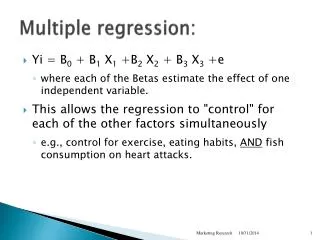
Multiple Regression Predicting a response with multiple explanatory variables
Assumptions • Sample representative • Error is random with mean of zero • Independent variables measured without error • Independent variables are linearly independent (multicollinearity) • Errors uncorrelated • Variance is constant (homoscedasticity
Data/Distribution Issues • Consideration of outlier values – accurate estimates may require eliminating them or using robust approaches • Non-normal distributions may require transformation • Plot response against each explanatory variable
Modeling • We want to obtain a model that fits the response (predicts) variable with as few variables as possible • R2 measures proportion of variability accounted for by the explanatory variables • Adjusted R2 takes the number of explanatory variables into account
Modeling Methods • General approach is to include variables theoretically relevant to predicting the response • Gradually remove variables that are not significant and compare difference between models for significance • Automatic stepwise methods • Forward and backwards
A Simple Example • Kalahari data includes site area (LMS), the number of days the site was occupied and the number of people who occupied it • Rcmdr – Statistics | Fit models | Linear Model
Two models • Model 1: LMS ~ People + Days • Model 2: LMS ~ People * Days • LMS ~ People + Days + People * Days • Check significance of slopes • Compare models for significant difference
> LinearModel.1 <- lm(LMS ~ People +Days, data=Kalahari) > summary(LinearModel.1) Call: lm(formula = LMS ~ People + Days, data = Kalahari) Residuals: Min 1Q Median 3Q Max -84.067 -8.387 1.395 19.792 60.233 Coefficients: Estimate Std. Error t value Pr(>|t|) (Intercept) -94.968 37.051 -2.563 0.0249 * People 12.276 2.062 5.953 6.68e-05 *** Days 5.885 1.992 2.954 0.0121 * --- Signif. codes: 0 '***' 0.001 '**' 0.01 '*' 0.05 '.' 0.1 ' ' 1 Residual standard error: 37.92 on 12 degrees of freedom Multiple R-squared: 0.8001, Adjusted R-squared: 0.7668 F-statistic: 24.02 on 2 and 12 DF, p-value: 6.377e-05
> LinearModel.2 <- lm(LMS ~ People*Days, data=Kalahari) > summary(LinearModel.2) Call: lm(formula = LMS ~ People * Days, data = Kalahari) Residuals: Min 1Q Median 3Q Max -85.921 -11.310 5.595 18.593 35.520 Coefficients: Estimate Std. Error t value Pr(>|t|) (Intercept) -5.1301 63.9905 -0.080 0.938 People 6.3835 4.0219 1.587 0.141 Days -6.6859 7.7606 -0.862 0.407 People:Days 0.8111 0.4862 1.668 0.123 Residual standard error: 35.38 on 11 degrees of freedom Multiple R-squared: 0.8405, Adjusted R-squared: 0.797 F-statistic: 19.32 on 3 and 11 DF, p-value: 0.0001083
> anova(LinearModel.1, LinearModel.2) Analysis of Variance Table Model 1: LMS ~ People + Days Model 2: LMS ~ People * Days Res.Df RSS Df Sum of Sq F Pr(>F) 1 12 17252 2 11 13768 1 3483.9 2.7834 0.1234
Darl Points • Create subset of DartPoints containing only the Darl Points • Model 1: Length ~ Width + Thickness • Model 2: Length ~ Width * Thickness
> LinearModel.4 <- lm(Length ~ Width +Thick, data=Darl) > summary(LinearModel.4) Call: lm(formula = Length ~ Width + Thick, data = Darl) Residuals: Min 1Q Median 3Q Max -9.297 -3.214 -1.250 4.592 7.449 Coefficients: Estimate Std. Error t value Pr(>|t|) (Intercept) 6.369 6.639 0.959 0.3470 Width 1.178 0.453 2.601 0.0157 * Thick 2.219 1.023 2.168 0.0403 * --- Signif. codes: 0 '***' 0.001 '**' 0.01 '*' 0.05 '.' 0.1 ' ' 1 Residual standard error: 4.652 on 24 degrees of freedom Multiple R-squared: 0.5418, Adjusted R-squared: 0.5037 F-statistic: 14.19 on 2 and 24 DF, p-value: 8.554e-05
> LinearModel.5 <- lm(Length ~ Width * Thick, data=Darl) > summary(LinearModel.5) Call: lm(formula = Length ~ Width * Thick, data = Darl) Residuals: Min 1Q Median 3Q Max -9.905 -2.728 -1.568 4.212 7.153 Coefficients: Estimate Std. Error t value Pr(>|t|) (Intercept) -30.4873 51.6259 -0.591 0.561 Width 3.2605 2.9281 1.114 0.277 Thick 7.8492 7.8883 0.995 0.330 Width:Thick -0.3135 0.4354 -0.720 0.479 Residual standard error: 4.699 on 23 degrees of freedom Multiple R-squared: 0.5519, Adjusted R-squared: 0.4935 F-statistic: 9.444 on 3 and 23 DF, p-value: 0.000296
> anova(LinearModel.4, LinearModel.5) Analysis of Variance Table Model 1: Length ~ Width + Thick Model 2: Length ~ Width * Thick Res.Df RSS Df Sum of Sq F Pr(>F) 1 24 519.33 2 23 507.88 1 11.447 0.5184 0.4788

