Download
1 / 7
70 likes | 139 Vues
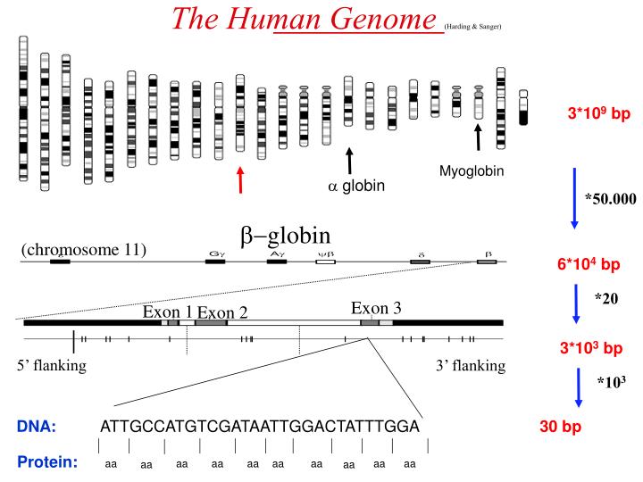
The Human Genome (Harding & Sanger). 3*10 9 bp. Myoglobin. a globin. *50.000. b- globin. (chromosome 11). 6*10 4 bp. *20. Exon 3. Exon 1. Exon 2. 3*10 3 bp. 5’ flanking. 3’ flanking. *10 3. DNA:. ATTGCCATGTCGATAATTGGACTATTTGGA. 30 bp. Protein:. aa. aa. aa. aa. aa. aa.

E N D
The Human Genome (Harding & Sanger) 3*109 bp Myoglobin a globin *50.000 b-globin (chromosome 11) 6*104 bp *20 Exon 3 Exon 1 Exon 2 3*103 bp 5’ flanking 3’ flanking *103 DNA: ATTGCCATGTCGATAATTGGACTATTTGGA 30 bp Protein: aa aa aa aa aa aa aa aa aa aa
Models of substitution I : Basic Models 15.10 Models of substitution II : Complex Models 16.10 Models of substitution III : Advanced Questions 22.10 A 1 2 3 5 4 T Phylogenies I: Combinatorics 23.10 Phylogenies II: Parsimony 29.10 Phylogenies III: Likelihood 30.10 Phylogenies IV: Inference 5.11 Networks I: Dynamics 6.11 Networks II: Inference 12.11 Networks III: Evolution 13.11 Schedule Alignment Algorithms I Optimisation 19.11 (Rune) Alignment Algorithms II Statistical Inference 20.11 (Rune) ACT-T -GTCT Stochastic Grammars and their Biological Applications: Hidden Markov Models 26.11 Finding Signals in Sequences 27.11 RNA structures (Rune) 3.12 Finding Recombinations in Sequences 4.12 Projects in substitution models, phylogenies, networks, grammars, RNA structure, signals, your choice Course should appeal to combinatorics, probability theory, statistics, algorithmics, software design, Summer projects: http://www.stats.ox.ac.uk/research/genome/projects EMAILS: lyngsoe@stats.ox.ac.ukhein@stats.ox.ac.ukmitchell@stats.ox.ac.uk
ACGCC ACGCC AGGCC AGGCC AGGCT AGGCT AGGGC AGGCT AGGCT AGGTT AGGTT AGTGC Central Problems: History cannot be observed, only end products. ACGTC ACGTC Even if History could be observed, the underlying process couldn’t !!
Some Definitions State space – a set often corresponding of possible observations ie {A,C,G,T}. A random variable, X can take values in the state space with probabilities ie P{X=A} = ¼. The value taken often indicated by small letters - x Stochastic Process is a set of time labeled stochastic variables Xt ie P{X0=A, X1=C, .., X5=G} =.00122 Time can be discrete or continuous, in our context it will almost always mean natural numbers, N {0,1,2,3,4..}, or an interval on the real line, R. Markov Property: ie Time Homogeneity – the process is the same for all t.
Simplifying Assumptions I Probability of Data Biological setup TCGGTA TGGTT a - unknown 1) Only substitutions. s1 TCGGTA s1 TCGGA s2 TGGT-T s2 TGGTT a5 a4 a3 a2 a1 T A T G G G G C T T Data: s1=TCGGTA,s2=TGGTT 2) Processes in different positions of the molecule are independent, so the probability for the whole alignment will be the product of the probabilities of the individual patterns.
Simplifying Assumptions II a l2+l1 l1 = l2 N1 N2 N2 N1 3) The evolutionary process is the same in all positions 4) Time reversibility: Virtually all models of sequence evolution are time reversible. I.e. πi Pi,j(t) = πj Pj,i(t), where πi is the stationary distribution of i and Pt(i->j) the probability that state i has changed into state j after t time. This implies that
Simplifying assumptions III t1 e A t2 C C 5) The nucleotide at any position evolves following a continuous time Markov Chain. Pi,j(t) continuous time markov chain on the state space {A,C,G,T}. Q - rate matrix: T O A C G T FA -(qA,C+qA,G+qA,T) qA,C qA,G qA,T RC qC,A -(qC,A+qC,G+qC,T) qC, G qC ,T OG qG,A qG,C -(qG,A+qG,C+qG,T) qG,T MT qT,A qT,C qT,G -(qT,A+qT,C+qT,G) 6) The rate matrix, Q, for the continuous time Markov Chain is the same at all times (and often all positions). However, it is possible to let the rate of events, ri, vary from site to site, then the term for passed time, t, will be substituted by ri*t.