CS 6463: AT Computational Geometry Fall 2006
50 likes | 198 Vues
CS 6463: AT Computational Geometry Fall 2006. Expected Runtimes Carola Wenk. Probability. Let S be a sample space of possible outcomes. E S is an event The (Laplacian) probability of E is defined as P( E )=| E |/| S | P( s )=1/| S | for all s S.

CS 6463: AT Computational Geometry Fall 2006
E N D
Presentation Transcript
CS 6463: AT Computational GeometryFall 2006 Expected Runtimes Carola Wenk CS 6463: AT Computational Geometry
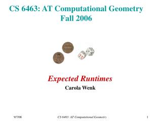
Probability • Let S be a sample space of possible outcomes. • ES is an event • The (Laplacian) probability of E is defined as P(E)=|E|/|S| P(s)=1/|S| for all sS Note: This is a special case of probability distribution. In general P(s) can be quite arbitrary. For a loaded die the probabilities could be for example P(6)=1/2 and P(1)=P(2)=P(3)=P(4)=P(5)=1/10. Example: Rolling a (six-sided) die • S = {1,2,3,4,5,6} • P(2) = P({2}) = 1/|S| = 1/6 • Let E ={2,6}P(E) = 2/6 = 1/3 = P(rolling a 2 or a 6) In general: For any sS and any ES • 0 P(s) 1 • P(s) = 1 • P(E) = P(s) sS sE CS 6463: AT Computational Geometry
Random Variable Head • A random variable X is a function from S to RX: S→ R Tail Head Example 1: Flip coin three times. • S = {HHH, HHT, HTH, HTT, THH, THT, TTH, TTT} • Let X(s) = # heads ins X(HHH) = 3X(HHT)=X(HTH)=X(THH) = 2X(TTH)=X(THT)=X(HTH) = 1X(TTT) = 0 Example 2: Play game: Win $5 when getting HHH, pay $1 otherwise • Let Y(s) be the win/loss for the outcomes Y(HHH) = 5Y(HHT) = Y(HTH) = … = -1 What is the average win/loss? CS 6463: AT Computational Geometry
Expected Value Notice the similarity to the arithmetic mean (or average). sS xR • The expected value of a random variable X: S→Ris defined asE(X) = P(s) X(s) = P({X=x}) x Example 2 (continued): • E(Y) = P(s) Y(s) = P(HHH) 5 + P(s) (-1) = 1/23 5 + 7 1/23 (-1) = (5-7)/23 = -2/8 = -1/4 = P({Y=y}) y = P(HHH) 5 + P(HHT) (-1) + P(HTH) (-1) + P(HTT) (-1) + P(THH) (-1) + P(THT) (-1) + P(TTH) (-1) + P(TTT) (-1) The average win/loss is E(Y) = -1/4 sS sS\{HHH} xR Theorem (Linearity of Expectation): Let X,Ybe two random variables onS. Then the following holds:E(X+Y) = E(X) + E(Y) Proof: E(X+Y) = P(s) (X(s)+Y(s)) = P(s)X(s) + P(s)Y(s) = E(X) + E(Y) sS sS sS CS 6463: AT Computational Geometry
Randomized algorithms • Allow random choices during the algorithm • Sample space S = {all sequences of random choices} • The runtime T: S→Ris a random variable. The runtime T(s) depends on the particular sequence s of random choices. Consider the expected runtimeE(T) Example 3 (Trapezoidal map): • The runtime depends on the order in which trapezoids are inserted: • ki = # new trapezoids created; total runtime is i=1 ki • Worst case: ki=O(i)Total worst-case runtime isi=1i= O(n2) • Best case: ki=O(1)Total worst-case runtime isi=1 1= O(n) • Insert segments in random order: • P = {all possible permutations/orders of segments}; |P| = n! for n segments • ki = ki(p) for some random order pP • E(ki)=O(1)(see theorem on slides) • Expected runtimeE(T) = E(i=1ki)=i=1E(ki)= O(i=11)= O(n) n n n n n n linearity of expectation CS 6463: AT Computational Geometry
