Download
1 / 39
390 likes | 570 Vues
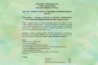
NUMERICAL METHODS THAT CAN BE USED IN BIOMECHANICS. Mechanics of Materials Approach (A) Complex Beam Theory (i) Straight Beam (ii) Curved Beam (iii) Composite Beam. From:Daviddarling.info. NUMERICAL METHODS THAT CAN BE USED IN BIOMECHANICS. Mechanics of Material Approach (Cont).

E N D
NUMERICAL METHODS THAT CAN BE USED IN BIOMECHANICS • Mechanics of Materials Approach (A) Complex Beam Theory (i) Straight Beam (ii) Curved Beam (iii) Composite Beam From:Daviddarling.info
NUMERICAL METHODS THAT CAN BE USED IN BIOMECHANICS Mechanics of Material Approach (Cont)
NUMERICAL METHODS THAT CAN BE USED IN BIOMECHANICS (2) Finite Difference Method
NUMERICAL METHODS THAT CAN BE USED IN BIOMECHANICS (2) Finite Difference Method (Contd) Consider an ordinary differential equation One of the difference equation method is using: To approximate the differential equation. Solution is:
Introduction • Re-invented around 1963 • Initially applied to engineering structures Concrete dams Aircraft structures (Civil engineers) (Aeronautical engineers)
Introduction • FEM is based on Energy Method Method of Residuals
Introduction • Energy method Total potential energy must be stationary δ (U + W) = δ ( П ) = 0
Introduction • Residual method Differential equation governing the problem is given by A ( ø ) = 0 Minimise R = A ( ø* ) - A ( ø ) ø is actual solution ø* is assumed solution
Introduction • Both methods give us a set of equations [ K ] { a } = { f } Stiffness Matrix Force Matrix Displacement Matrix
Introduction - FEM Procedure • Continuum is separated by imaginary lines or surfaces into a number of “finite elements” Finite Elements
Introduction - FEM Procedure • Elements are assumed to be interconnected at a discrete number of “nodal points” situated on their boundaries Nodal Points Finite Elements Displacements at these nodal points will be the basic unknown
Introduction - FEM Procedure • A set of functions is chosen to define uniquely the state of displacement within each finite element ( U ) in terms of nodal displacements ( a1 , a2 , a3 ) Finite Element a2 Nodal Point U = Σ Ni ai i= 1, 3 y a3 a1 x
Introduction - FEM Procedure • This displacement function is input into either “energy equations” or “residual equations” to give us element equilibrium equation • [ K ] { a } = { f } Finite Element a2 Nodal Point y Element Displacement Matrix Element Force Matrix Element Stiffness Matrix a3 a1 x
Introduction - FEM Procedure • Element equilibrium equations are assembled taking care of displacement compatibility at the connecting nodes to give a set of equations that represents equilibrium of the entire continuum Nodal Points Finite Elements
Introduction - FEM Procedure • Solution for displacements are obtained after substituting boundary conditions in the continuum equilibrium equations Nodal Points Finite Elements Support Points Support Points
Introduction • Finite element method used to solve: • Elastic continuum • Heat conduction • Electric & Magnetic potential • Non-linear (Material & Geometric) -plasticity, creep • Vibration • Transient problems • Flow of fluids • Combination of above problems • Fracture mechanics
Introduction • Finite elements: • Truss , Cable and Beam elements • Two & Three solid elements • Axi-symmetric elements • Plate & Shell elements • Spring, Damper & Mass elements • Fluid elements
Finite Element Mesh of C4-C7 Facet Joints C4 C5-C6 Graft C5 C6 C7 Intact With Graft at C5-C6 Level
von Mises Stress in C4-C5 Annulus (Flexion) 5 MPa Anterior 6 MPa Anterior Kyphotic Graft Neutral Graft
Vertical Displacement Distribution in L1-S1
Finite Element Mesh of L2-L5 With 25% Translational Spondylolisthesis
Vertical Displacement Distribution in L2-L5 Under Flexion Moment (25% translational spondylolisthesis)
Finite Element Mesh to Represent Tibial Insert & Femoral Component
Motion of Femoral Implant with respect to UHMWPE Knee Insert
SIGMA-ZZ in cortical bone in a femur with implant attached using cement
Advantage of using FEM • Irregular complex geometry can be modeled • Effect of large number of variables in a problem can be easily analysed • Multiple phase problems can be modeled • Effect of various surgical techniques can be compared using appropriate FE models • Both static and time dependent problems can be modeled • Solution to certain problems that cannot be (or difficult) obtained otherwise can be solved by FEM