Computational Spectroscopy Introduction and Context
200 likes | 387 Vues
Computational Spectroscopy Introduction and Context. Chemistry 713 (a) What is spectroscopy? (b) Model Chemistries. What is Spectroscopy?. A plot of light intensity or power as a function of frequency, , or wavelength,

Computational Spectroscopy Introduction and Context
E N D
Presentation Transcript
Computational SpectroscopyIntroduction and Context Chemistry 713 (a) What is spectroscopy? (b) Model Chemistries
What is Spectroscopy? • A plot of light intensity or power as a function of frequency, , or wavelength, • Speed of light in a material with index of refraction n is c/n=. (n=1 in a vacuum.) • Emission or absorption of light by atoms and molecules depends on frequency. • For absorption and emission, the energy of a photon of light E=h is equal to the difference in energy between molecular energy levels: h = E2 - E1 • For scattering, both energy and momentum (p=h/) are conserved. • In certain circumstances, electrons or other particles (=h/p) are used instead of photons.
A linear absorption spectrum of methylamine (wavenumber is ) What kinds of spectroscopy? • Linear spectroscopy • Spectral intensities are proportional to the intensity of the light at the indicated frequency. • Nonlinear spectroscopies • Spectral intensities are NOT proportional to the intensity of the light at the indicated frequency, or • Spectral intensities depend on the light intensities at more than one frequency. (e.g., 2-D and 3-D spectroscopies).
What kinds of molecular motions? • Rotational spectra (gas phase) • Determined by molecular geometry • Microwave and far infrared regions. • Vibrational spectra • The electronic wavefunctions determine the chemical bonding, which in turn determines the force constants between the atoms and hence the vibrational frequencies. • Accompanied by rotational transitions (gas phase). • Absorption in the infrared region and Raman scattering. • Electronic Spectra • Transitions between electronic states are accompanied by vibrational and rotational transitions. • Visible and ultraviolet regions
Spectra from intrinsic spin • Nuclear magnetic resonance (NMR) spectroscopy • Nuclear spins (I>0), when placed in a magnetic field, can have only certain orientations relative to the magnetic field and these orientations have different energies. • Transitions between these energy levels, typically in the radio frequency region, give rise to NMR spectra. • Electron spin resonance (ESR) spectroscopy • Molecules with unpaired electron spins • Transitions between different orientations of electronic angular momenta are in the microwave region for typical magnetic fields. • This course will focus on rotational, vibrational, and electronic spectra, but projects on NMR spectra are possible.
Diffraction of X-rays and electrons • Measurement of scattered intensities vs scattering angle. • Relies on conservation of momentum rather than energy. • Provides information about the relative positions of atoms in condensed phases. • X-ray diffractions of crystalline • solids gives precise relative geometries of atoms (Youngs’ course 3150:645). • X-ray diffraction of liquids, polymers, and amorphous materials gives the pair distribution function. • Low energy electron diffraction (LEED) gives the structure of ordered surfaces. • Electron diffraction can give the structure of isolated gas molecules. • Diffraction per se is not covered in this course, but we will compute molecular geometries.
Computation of Spectra • First calculate the relevant molecular properties: • Molecular geometry for rotational spectra • Force constants for vibrational spectra • Electronic energy states for electronic spectra. • Second, use this information to calculate transition frequencies and intensities, that can be compared to experiment.
Why bother to compute molecular spectra? • Spectroscopy is our most powerful means of gaining information about the molecular world. • Molecular structure and properties • Molecular dynamics • Chemical reactions, energy transfer, protein folding, … • Detection and quantification of molecular species • The desired information is not given directly, but is coded in the spectra, often in a complicated way. • Computation of spectra helps to break the code. • Provide a deeper understanding than allowed by “rule of thumb” interpretations of spectra. • Computational methods are now exceptionally powerful and are increasingly accessible to every chemist.
Model Chemistries • A computational model is defined by the concepts and assumptions that go into it. • Ideally defined in a general way that could be applied to any chemical system, and reproducible by any user. • Specifically, the means used to calculate the molecular structure, properties, and potential energy surface(s). • Molecular mechanics • Electronic structure methods • Semi-empirical methods • Density functional theory • Ab initio methods Foresman & Frisch, pp 3ff
Model Chemistries Molecular Mechanics • Based on an empirical potential energy hypersurface that determines the forces exerted on the atoms in any particular molecular geometry.1 • V(x1,x2,…x3N) is given by an equation involving • the distances and angles between the N atoms • the atom types, e.g., H, C(sp3), C(sp2), Ca++, etc. • a set of parameters estimated from experimental data • includes covalent, electrostatic, and van der Waals interactions, and possible solvent effects • defined in Sybyl, AMBER, MM3 2, CHARM 3, etc. software packages From the front cover of “Energy Landscapes with Applications to Clusters, Biomolecules, and Glasses”, by David J. Wales, Cambridge University Press, 2003 1. There is a great description of the molecular mechanics method by John Wampler of the U of Georgia on the web at www.bmb.uga.edu/wampler/399/lectures/mm1 2. Allinger, N. L., Yuh, Y. H., & Lii, J-H. (1989) Molecular Mechanics. The MM3 Force Field for Hydrocarbons. 1. J. Am. Chem. Soc. 111, 8551-8565. 3. Brooks, B.R., Bruccoleri, R.E., Olafson, B.D., States, D.J., Swaminathan, S., Karplus, M. CHARMM: A program for macromolecular energy, minimization, and dynamics calculations. J. Comp. Chem. (1983) 4, 187-217.
Model Chemistries Molecular Mechanics • Complicated molecules may have dozens, thousands, or millions of minima. • How do we find “the real structure”? • The biologically active form of a protein may or may not be the global minimum structure. • Often molecules are dynamic, sampling multiple conformations during a process of interest. • To find “the” molecular structure: • Start the molecule relatively hot, so that it can get over the various saddle points. • Integrate the equations of motion of the atoms by classical mechanics for a LONG time. • Assume that the molecules sample all of the relevant geometries during that time. (ergodic assumption) • Gradually take away energy (anneal it) until the molecule settles down into one or a few geometries. Fig. 5.4, p 252 from Wales. On left are 1-D potential energy surfaces, and on left are the corresponding “disconnectivity” graphs.
Model Chemistries Molecular Mechanics • Advantages • Very large systems can be treated because classical mechanics is efficient and the computational effort for sufficiently systems scales linearly with the system size.1 • Pitfalls • The empirical • force field may not be calibrated for the system type of interest, nor sufficiently accurate for the properties of interest. • The ergodic hypothesis may fail and consequently, the global minimum or other important conformations may not be found. 1. C. J. Cramer, Essentials of Computational Chemistry - Theories and Models, Wiley 2004, p 14.
Model Chemistries Electronic Structure Methods • Semi-empirical methods • Some quantum mechanics + experimental data • Density Functional Theory (DFT) • Quantum mechanics + empirical exchange and correlation functionals • Almost an ab initio method • Ab initio methods • ab initio = “from the beginning” • Relies only on quantum mechanics + a small number of fundamental constants: • h, c, and masses & charges of electrons and nuclei
Model Chemistries - Electronic Structure Methods Semi-empirical Methods • A very simplified quantum treatment of the bonding • The needed integrals are not evaluated explicitly, but are treated as parameters to be calibrated from experimental data on reference systems. • Hückel theory treats only the electrons and the strength of the interaction between adjacent p orbital is taken as a parameter that can be varied to fit experimental data. • Gives a qualitative, and often semi-quantitative, treatment of aromaticity. • More sophisticate semi-empirical methods, e.g., AMI, MINDO/3, PM3, are included in such packages as Gaussian, Spartan, and HyperChem. • Not extensively used any more because • DFT is reasonably fast even for fairly large systems • Faster computers have made DFT and ab initio method tractable for larger systems • For very large systems empirical potentials are now better parametrized.
Ru(terpy)2 dimer HOMO Empirical + ab initio MM2 geometry; HF/3-21G Orbital
Model Chemistries - Electronic Structure Methods Density Functional Theory (DFT) • Strategy is to model electron correlation via general functionals of the electron density. • A functional is a function whose definition is also a function, that is, a function of a function. • Hohenberg-Kohn theorem (Phys. Rev. 136, B864 (1964)) says that the ground state energy is equal to a functional of the electron density: E0=E0[0] • The problem is that it doesn’t tell us what the functional is, so we have to guess. • Strategy: calculate the energy without electron correlation first by ab initio means (Hartree-Fock (HF)). • Then use the resulting wavefunctions to get the electron density and come up with a functional to treat only the contribution of electron correlation. • Some functionals depend only on the local density (Local Density Approximation (LDA)); others include the gradient of the density at each point. (gradient-corrected functionals). • In practice DFT calculations are not done just as a single step, but uses an iterative approach analogous to the Hartree-Fock self-consistent field method. • The Becke 3 - Lee, Yang, Parr (B3LYP) functional is one of the most popular. • Many new functionals are reported in the literature. • The computer time required is only a little longer than Hartree-Fock - if it is coded efficiently.
Model Chemistries - Electronic Structure Methods ab initio Methods • For a given molecular geometry (i.e., fixed nuclear coordinates, R), solve the electronic Schroedinger equation: where He is the whole molecular Hamiltonian except the nuclear kinetic energy and r represents the coordinates for all of the electrons, and e is the electronic wave function. Repeat for all molecular geometries R of interest. • This is called the Born-Oppenheimer approximation, and the relevant theory can be found in Ira N. Levine, Quantum Chemistry, 5th ed, Prentice Hall (2000). • The B.O. approx. is not perfect, but it is always used, at least as a starting point, because we are helpless without it. • The nuclear motion can then be solved as a separate step. The electronic energy E(R) is the potential energy in which the nuclei move. • The electronic Schroedinger equation is too difficult to be solve exactly, so approximate methods must be used.
Model Chemistries - Electronic Structure Methods ab initio Methods • The repulsion between electrons is the term that causes the most problem. This means that the motions of the electrons are intricately correlated in a very complicated way. • As a practical matter, we still treat one electron at a time, moving in the average field of the other electrons: • Start by guessing the wavefunction of each electron, and use it to calculate the average repulsive field of each electron. • One at a time, solve for the wavefunctions of each electron to get better 1-electron wavefunctions. • Recalculate the average repulsive field of each electron, and repeat the process until a self-consistent field is obtained. • When the effects of the Pauli Principle (exchange interactions) are included, this is call the Hartree-Fock Self-Consistent Field (HF) method. • The fact that electron motions are correlated is completely neglected by the HF method.
Model Chemistries - Electronic Structure Methods ab initio Methods • More advanced methods treat electron correlation at some level of approximation. • DFT - quick, but we have to guess what density functional to use. • MP2 - Möller-Plesset Perturbation Theory • Electron correlation is treated by 2nd order perturbation theory • MP4 - Möller-Plesset Perturbation Theory, 4th order • QCISD(T) - quadratic configuration interaction including single and double excitations, and with triples treated perturbatively. • Multiple electron configurations can be included to account for electron correlation. • VERY time consuming. • CCSD(T) - coupled cluster theory including single and double excitations, and with triples treated perturbatively. • Faster than QCISD(T) • Sometimes called “the gold standard” for single reference problems. • CASSCF - multi-reference method • Good when multiple inequivalent resonance hybrids are important. • CASPT2 - a multi reference method with electron with a perturbative treatment of electron correlation.
Model Chemistries - Electronic Structure Methods ab initio Methods • Even for the Hartree-Fock method, we can’t solve the electronic Schroedinger equation exactly. • Express the wavefunction for each electron as a linear combination of atomic-like orbitals on each atom - called the “basis set”- then use variation method. • Just like vectors in 3-dimensions are expressed as linear combinations of the i, j, k unit vectors • Wavefunctions are VECTORS in an infinite dimensional vector space. • Approximate with a finite number of basis vectors (= functions). • The Hamiltonian becomes a MATRIX, that we will DIAGONALIZE to find approximate eigenvalues (energies) and eigenvectors (wavefunctions). • Available basis sets include • Split-valence basis sets: 3-21G, 6-31G*, 6-311++G**, etc • Dunning correlation-consistent basis sets: cc-pVDZ, aug-cc-pVTZ, etc • The larger the basis set, the more accurate the result and the more computer time required.