Download
1 / 78
800 likes | 970 Vues
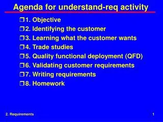
Agenda for understand req activity. 1. Numbers 2. Decibels 3. Matrices 4. Transforms 5. Statistics 6. Software. 1. Numbers. Significant digits Precision Accuracy. 1. Numbers. Significant digits (1 of 5).

E N D
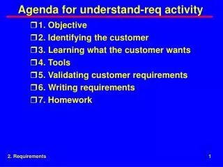
Agenda for understand req activity • 1. Numbers • 2. Decibels • 3. Matrices • 4. Transforms • 5. Statistics • 6. Software
1. Numbers • Significant digits • Precision • Accuracy 1. Numbers
Significant digits (1 of 5) • The significant digits in a number include the leftmost, non-zero digits to the rightmost digit written. • Final answers should be rounded off to the decimal place justified by the data 1. Numbers
Significant digits (2 of 5) Examples number digits implied range 251 3 250.5 to 251.5 25.1 3 25.05 to 25.15 0.000251 3 0.0002505 to 0.0002515 251x105 3 250.5x10⁵ to 251.5x10⁵ 2.51x10⁻³ 3 2.505x10⁻³ to 2.515x10⁻³ 2510 4 2509.5 to 2510.5 251.0 4 250.95 to 251.05 1. Numbers
Significant digits (3 of 5) • Example • There shall be 3 brown eggs for every 8 eggs sold. • A set of 8000 eggs passes if the number of brown eggs is in the range 2500 to 3500 • There shall be 0.375 brown eggs for every egg sold. • A set of 8000 eggs passes if the number of brown eggs is in the range 2996 to 3004 1. Numbers
Significant digits (4 of 5) • The implied range can be offset by stating an explicit range • There shall be 0.375 brown eggs (±0.1 of the set size) for every egg sold. • A set of 8000 eggs passes if the number of brown eggs is in the range 2200 to 3800 • There shall be 0.375 brown eggs (±0.1) for every egg sold. • A set of 8000 eggs passes only if the number of brown eggs is 3000 1. Numbers
Significant digits (5 of 5) • A common problem is to inflate Significant digits in making units conversion. • Observers estimated the meteorite had a mass of 10 kg. This statement implies the mass was in the range of 5 to 15 kg; i.e, a range of 10 kg. • Observers estimated the meteorite had a mass of 22 lbs. This statement implies a range of 21.5 to 22.5 lb; i.e., a range of 1 pound 1. Numbers
Precision • Precision refers to the degree to which a number can be expressed. • Examples • Computer words • The 16-bit signed integer has a normalized precision of 2-15 • Meter readings • The ammeter has a range of 10 amps and a precision of 0.01 amp 1. Numbers
Accuracy • Accuracy refers to the quality of the number. • Examples • Computer words • The 16-bit signed integer has a normalized precision of 2-15,but its normalized accuracy may be only ±2-3 • Meter readings • The ammeter has a range of 10 amps and a precision of 0.01 amp, but its accuracy may be only ±0.1 amp. 1. Numbers
2. Decibels • Definitions • Common values • Examples • Advantages • Decibels as absolute units • Powers of 2 2. Decibels
Definitions (1 of 2) • The decibel, named after Alexander Graham Bell, is a logarithmic unit originally used to give power ratios but used today to give other ratios • Logarithm of N • The power to which 10 must be raised to equal N • n = log10(N); N = 10n 2. Decibels
Definitions (2 of 2) • Power ratio • dB = 10 log10(P2/P1) • P2/P1=10dB/10 • Voltage power • dB = 10 log10(V2/V1) • P2/P1=10dB/20 2. Decibels
Common values dB ratio 0 1 1 1.26 2 1.6 3 2 4 2.5 5 3.2 6 4 7 5 8 6.3 9 8 10 10 100 20 1000 30 2. Decibels
Examples • 5000 = 5 x 1000; 7 dB + 30 dB = 37 dB • 49 dB = 40 dB + 9 dB; 8 x 10,000 = 80,000 2. Decibels
Advantages (1 of 2) • Reduces the size of numbers used to express large ratios • 2:1 = 3 dB; 100,000,000 = 80 dB • Multiplication in numbers becomes addition in decibels • 10*100 =1000; 10 dB + 20 dB = 30 dB • The reciprocal of a number is the negative of the number of decibels • 100 = 20 dB; 1/100 = -20 dB 2. Decibels
Advantages (2 of 2) • Raising to powers is done by multiplication • 1002 = 10,000; 2*20dB = 40 dB • 1000.5 = 10; 0.5*20dB = 10 dB • Calculations can be done mentally 2. Decibels
Decibels as absolute units • dBW = dB relative to 1 watt • dBm = dB relative to 1 milliwatt • dBsm = dB relative to one square meter • dBi = dB relative to an isotropic radiator 2. Decibels
Powers of 2 exact value approximate value 20 1 1 24 16 16 210 1024 1 x 1,000 223 8,388,608 8 x 1,000,000 234 17,179,869,18416 x 1,000,000,000 2xy = 2y x 103x 2. Decibels
3. Matrices • Addition • Subtraction • Multiplication • Vector, dot product, & outer product • Transpose • Determinant of a 2x2 matrix • Cofactor and adjoint matrices • Determinant • Inverse matrix • Orthogonal matrix 3. Matrices
Addition C=A+B 1 -1 -1 0 4 2 -1 0 1 2 -2 -1 -2 5 -1 1 0 3 1 -1 0 -2 1 -3 2 0 2 A= B= C= cIJ = aIJ + bIJ 3. Matrices
Subtraction C=A-B 1 -1 -1 0 4 2 -1 0 1 0 0 1 -2 -3 -5 3 0 1 1 -1 0 -2 1 -3 2 0 2 A= B= C= cIJ = aIJ - bIJ 3. Matrices
Multiplication C=A-B 1 -1 -1 0 4 2 -1 0 1 1 -5 -3 1 6 1 0 -2 0 1 -1 0 -2 1 -3 2 0 2 A= B= C= cIJ = aI1 * b1J + aI2 * b2J + aI3 * b3J 3. Matrices
Vector, dot product, & outer product • A vector v is an N x 1 matrix • Dot product = inner product = vT x v = a scalar • Outer product = v x vT = N x N matrix 3. Matrices
Transpose B=AT 1 -2 2 -1 1 0 0 -3 2 1 -1 0 -2 1 -3 2 0 2 A= B= bIJ = aJI 3. Matrices
Determinant of a 2x2 matrix 1 -1 -2 1 B = = -1 2x2 determinant = b11 * b22 - bI2 * b21 3. Matrices
Cofactor and adjoint matrices 1 -1 0 -2 1 -3 2 0 2 A= 1 -3 0 2 -2 -3 2 2 -2 1 2 0 2 -2 -2 2 2 -2 3 3 -1 -1 0 0 2 1 0 2 2 1 -1 2 0 B = cofactor = = -1 0 0 -3 1 0 -2 -3 1 -1 -2 1 2 2 3 -2 2 3 -2 -2 -1 C=BT = adjoint= 3. Matrices
Determinant 1 -1 0 -2 1 -3 2 0 2 determinant of A = =4 1 -1 0 2 -2 -2 = 4 The determinant of A = dot product of any row in A times the corresponding row the adjoint matrix = dot product of any row or column in A times the corresponding row or column in the cofactor matrix 3. Matrices
Inverse matrix 0.5 0.5 0.75 -0.5 0.5 0.75 -0.5 -0.5 -0.25 B = A-1 =adjoint(A)/determinant(A) = 1 -1 0 -2 1 -3 2 0 2 0.5 0.5 0.75 -0.5 0.5 0.75 -0.5 -0.5 -0.25 1 0 0 0 1 0 0 0 1 = 3. Matrices
Orthogonal matrix • An orthogonal matrix is a matrix whose inverse is equal to its transpose. 1 0 0 0 cos sin 0 -sin cos 1 0 0 0 cos -sin 0 sin cos 1 0 0 0 1 0 0 0 1 = 3. Matrices
4. Transforms • Definition • Examples • Time-domain solution • Frequency-domain solution • Terms used with frequency response • Power spectrum • Sinusoidal motion • Example -- vibration 4. Transforms
Definition • Transforms -- a mathematical conversion from one way of thinking to another to make a problem easier to solve problem in original way of thinking solution in original way of thinking transform solution in transform way of thinking inverse transform 4. Transforms
Examples (1 of 3) problem in English solution in English English to algebra solution in algebra algebra to English 4. Transforms
Examples (2 of 3) problem in English solution in English English to matrices solution in matrices matrices to English 4. Transforms
Examples (3 of 3) problem in time domain solution in time domain Fourier transform solution in frequency domain inverse Fourier transform • Other transforms • Laplace • z-transform • wavelets 4. Transforms
Time-domain solution • We typically think in the time domain -- a time input produces a time output input output amplitude amplitude system time time 4. Transforms
Frequency-domain solution (1 of 2) • However, the solution can be expressed in the frequency domain. • A sinusoidal input produces a sinusoidal output • A series of sinusoidal inputs across the frequency range produces a series of sinusoidal outputs called a frequency response 4. Transforms
Frequency-domain solution (2 of 2) input (sinusoids) output amplitude (dB) magnitude (dB) system log frequency log frequency phase (angle) 0 -180 log frequency 4. Transforms
Terms used with frequency response amplitude (dB) power (dB) • Octave is a range of 2x • Decade is a range of 10x 20,10 • Slope = • 20 dB/decade, amplitude • 6 dB/octave, amplitude • 10 dB decade, power • 3 dB decade, power 6, 3 2 10 frequency 4. Transforms
Power spectrum • A power spectrum is a special form of frequency response in which the ordinate represents power g2-Hz (dB) log frequency 4. Transforms
Sinusoidal motion • Motion of a point going around a circle in two-dimensional x-y plane produces sinusoidal motion in each dimension • x-displacement = sin(t) • x-velocity = cos(t) • x-acceleration = -2sin(t) • x-jerk = -3cos(t) • x-yank = 4sin(t) 4. Transforms
Example -- vibration transmissivity-squared input output g2-Hz (dB) amplitude (dB) g2-Hz (dB) log frequency log frequency log frequency Output vibration is product of input vibration times the transmissivity-squared at each frequency 4. Transforms
5. Statistics (1 of 2) • Frequency distribution • Sample mean • Sample variance • CEP • Density function • Distribution function • Uniform • Binomial 5. Statistics
5. Statistics (1 of 2) • Normal • Poisson • Exponential • Raleigh • Sampling • Combining error sources 5. Statistics
Frequency distribution • Frequency distribution -- A histogram or polygon summarizing how raw data can be grouped into classes number n = sample size = 39 8 6 4 2 2 2 4 5 7 4 6 6 3 2 60 61 62 63 64 65 66 67 68 height (inches) 5. Statistics
Sample mean N i=1 • = xi • An estimate of the population mean • Example N = [ 2 x 60 + 4 x61 + 5 x 62 + 7 x 63 + 4 x 64 + 6 x 65 + 6 x 66 + 3 x 67 + 2 x 68 ] / 39 = 2494/39 = 63.9 5. Statistics
Sample variance N i=1 N-1 • 2= (xi - )2 • An estimate of the population variance • = standard deviation • Example 2 = [ 2 x (60 - )2 + 4 x (61 - )2 + 5 x (62 - )2 + 7 x (63 - )2 + 4 x (64 - )2 + 6 x (65 - )2 + 6 x (66 - )2 + 3 x (67 - )2 + 2 x (68 - )2 ]/(39 - 1] = 183.9/38 = 4.8 = 2.2 5. Statistics
CEP • Circular error probable is the radius of the circle containing half of the samples • If samples are normally distributed in the x direction with standard deviation x and normally distribute in the y direction with standard deviation y , then CEP = 1.1774 * sqrt [0.5*(x2 + y2)] CEP 5. Statistics
Density function • Probability that a discrete event x will occur • Non-negative function whose integral over the entire range of the independent variable is 1 f(x) x 5. Statistics
Distribution function • Probability that a numerical event x or less occurs • The integral of the density function F(x) 1.0 x 5. Statistics
Uniform (1 of 2) • f(x) = 1/(x2 - x1 ), x1 x x2 = 0 elsewhere • F(x) = 0, x x1 = (x - x1 ) / (x2 - x1 ), x1 x x2 = 1, x > x2 • Mean = (x2 + x1 )/2 • Standard deviation = (x2 - x1 )/sqrt(12) 5. Statistics