Download
1 / 65
710 likes | 926 Vues
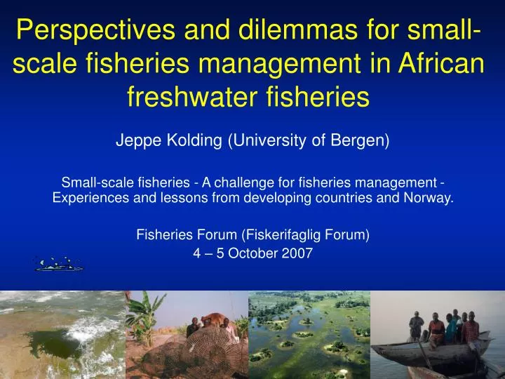
Perspectives and dilemmas for small-scale fisheries management in African freshwater fisheries. Jeppe Kolding (University of Bergen) Small-scale fisheries - A challenge for fisheries management - Experiences and lessons from developing countries and Norway.

E N D
Perspectives and dilemmas for small-scale fisheries management in African freshwater fisheries Jeppe Kolding (University of Bergen) Small-scale fisheries - A challenge for fisheries management - Experiences and lessons from developing countries and Norway. Fisheries Forum (Fiskerifaglig Forum) 4 – 5 October 2007
Background • Inland fisheries (and small-scale fisheries in general) are the ‘social security system’ in Africa – A common good! • Serves as the ‘last resort’ when everything else fail. • How should they be managed? • How can they be managed?
3 major dilemmas on small-scale fisheries management: • Why does the common property theory (CPT) only apply to man, and not to other predators? – they are also harvesting a common. • Why are we controlling effort increase (f), while we at the same time refine and develop the catchability (q)? • Why is man the only predator that has a harvesting pattern completely opposite all other predators?
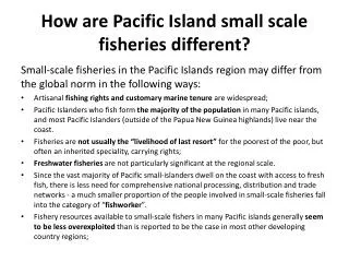
Small-scale fisheries comprise: • > 30 % of total world captures • > 50 % of total landings for human consumption • > 90 % of all fishermen • ≈ 80 % live in Asia Many ecosystems only exploitable on a small-scale • Coastal lagoons • Tidal flats, shallow shores • Estuaries • Coral reefs • Most freshwaters (contribute 25% of global production)
Marine and inland capture fisheries – top 10 producers 2002 China, India and Indonesia have populations of nearly 1 billion people living below the UNDP poverty line of US$ 1 per day (Staples et al. 2004) (SOFIA 2004)
Importance of fish for people The richer the less dependent on fish Relationship between the proportion of fish protein in human diets and the relative wealth (measured as GPD) of the nations they live in. From Kent (1998)
Small-scale fisheries • Research generally very, very small (mostly socio-economic) • Most fisheries biologist are dealing with large scale industrialized fisheries • Quantitative SSF data limited or nil • Problems and management? • copied from industrial fisheries (the ruling paradigm)
Small-scale fisheries • Mostly associated with developing countries • traditional - antiquated - primitive • poor - needs development • unmanaged - resource depleting - challenge • overfished • “Tragedy of the commons” • Having a negative image: • Illegal and destructive gears • Ignore regulations and legislation • Unruly members of society • Subject to “Maltusian” overfishing • “Poverty trap” • Unselective, indiscriminate fishing methods
Small-scale fisheries Thus, plenty of arguments for: They need to be managed! 90 % of projects use one or several of the above reasons for justifications But how to manage them? when: • Little research = little knowledge • Multi-species and multi-gear situations • Negligible monitoring • Unwillingness to abide • Costly to enforce The present answer (panacea) seems to be: Co-management and MPAs “They must learn to understand their own good” But do we understand their best ? Traditional fisheries management
Management paradigm The present mainstream research is focused on: • Industrial (valuable) fisheries • Single-species considerations • F, TAC, Quotas, size-limits • Enhanced selective harvesting strategies Purpose: A selective kill on targeted species and sizes Result: Dominate our thinking (paradigm) and forms our perception on small-scale fisheries • EAF (ecosystem approach to fisheries) is only recent on the agenda (Johannesburg 1992) and only conceptually debated = we don’t know how!
Patterns of exploitation Selectivity = rooted in all fisheries theory: • Mesh size regulations • Gear restrictions • By-catch • Destructive methods • seining • beat fishing • barriers, weirs • small mesh sizes In industrial fisheries non-selectivity = BAD Result: Universally applied - also in co-management! Almost universally banned in Africa
The selectivity paradigm • FAO 2003 (Ecosystem Approach to Fisheries): "Selectivity, or lack of it, is central to many biological issues affecting fisheries. Bycatch or incidental capture is responsible for endangering and contributing to extinction of a number of non-target species…. In addition, the discarding of unwanted catch, which is particularly important in unselective fisheries, is being considered by society not only as wasteful but as unethical. The Code of Conduct dedicates a whole section to the issue (8.5). It promotes the use of more selective gear (7.6.9; 8.4.5) and calls for more international collaboration in better gear development (8.5.1; 8.5.4), as well as for the agreement on gear research standards.”
SSF management = Copy+paste • Industrial fisheries are single species fisheries with single species management • They are so large and valuable that research and CMS is invested for management decisions • Small-scale fisheries are multi-species, multi-gear, too small to warrant research. • Our ‘understanding’ and assumptions on which we base our management is directly inherited from large-scale fisheries.
Q1: Why does the common property theory (CPT) only apply to man, and not to other predators? In the ‘balance of nature’ it is generally assumed that: • predation is the most important factor in natural mortality of fish (Sissenwine 1984; Vetter 1988; ICES 1988), • adaptations tend to maximize fitness through optimal utilization of resources (Slobodkin 1974; Stearns 1976; Maynard-Smith 1978), • predators and prey are co-evolved (Slobodkin 1974; Krebs 1985) and, • there is an uni-modal response of prey productivity to predator densities: (sigmoid curve theory = logistic Gordon Schaefer model)
Max = MSY No growth No surplus No stock No growth No surplus Stock = Max Logistic growth –Surplus production The rate of change in biomass production as a function of the biomass is uni-modal
Logistic growth - predator-prey • From above principles it is reasonable to assume that predation would 'maintain' prey populations close to their highest average production rate (Slobodkin 1961, 1968; Mertz & Wade 1976; Pauly 1979; Caddy & Csirke 1983; Carpenter et al. 1985). • The argument follows simply from the sigmoid curve where the highest surplus production of the prey population (dN/dt = max) is the 'carrying capacity' (K) of the predator population.
Predator-prey Thus predators can in theory grow to reach K (= MSYprey), but if they overshoot they will reduce prey production and consequently decline themselves. This is the background for density dependent cascade theory, and the coupled time-lagged oscillations observed between predator and prey
Predator-prey: Cascading effects Inverse biomass trends illustrating trophic cascades in the Black Sea (from Daskalov 2002)
What has this to do with CPT? • The big question is if effort is controlling the productivity or if the productivity is controlling the effort? Are small-scale fishermen different from other predators? • The answer to this dilemma is fundamental for applying CPT and co-management! • If we close for open access it will have severe consequences for the ‘last resort’ option • By closing open access we are in fact, closing the social security system of Africa!
Productivity in African lakes • Morphology • …of a lake, particularly area, volume, depth, and shoreline development or gradient, is of major importance to the productivity (Ryder 1978). • The mean depth encapsulates several of these attributes and is considered as the most important (Rawson 1952, Ryder et al. 1974, Mehner et al. 2005). • Nutrients • Lakes do not maintain fertility unless continual external loading of nutrients is applied (Schindler 1978, Moss 1988, Karenge and Kolding 1995). Water inflow is a major contributor and serves as a proxy for nutrient load. • Hydrology • The ‘flood pulse advantage’ is the amount by which fish yield per unit mean water area is increased by a natural, predictable flood pulse (Bayley 1991). The ‘flood pulse’ keeps the environment in a stage of early succession, which means that it is dominated by biota with r-selected traits (Junk et al. 1989).
The physical basis for lake productivity Not considered here Generalised effects of climatic, morphological, edaphic and hydrological factors (X-axis) on productivity (Y-axis)
Relative Lake Level Fluctuation Index (RLLF) … • …encapsulates the morphological, edaphic and hydrological driving forces for productivity into a single quantity. • … is a dynamic extension of the MEI index that only incorporated morphological and edaphic factors • … builds on the ‘flood pulse’ concept(Junk et al. 1989) and the ‘flood pulse advantage’ (Bayley 1991)
Hydrology and fish yields • Variability around the trend of total inland catches of the SADC countries show decadal fluctuations possibly influenced by long term climate variations (water levels)
Lake levels as drivers of fish productivity • Mean annual catch rates varies with water levels in most African fisheries. This has long been known by local fishermen, but not much investigated. Lake Kariba 1982-1992 Karenge and Kolding (1995) Lake Turkana 1972-1989 Kolding (1992)
Data on catch, effort and water levels • 17 major lakes and reservoirs in Africa. • Monthly time series (Min # years = 9) of lake levels from gauge readings (N = 13) or satellites (N = 4) • ESAhttp://earth.esa.int/riverandlake/ • TOPEX-POSEIDON http://www.pecad.fas.usda.gov/cropexplorer/global_reservoir/ • Yield and effort estimates from 1990’s (Updated from Jul-Larsen et al. (2003) and various projects we have been involved with). Kolding and van Zwieten (2007)
Lake Area km2 Mean depth m #Species Yield ton/yr #Fishermen RLLF annual RLLF seasonal Tanganyika 32600 580 240 73000 40000 0.04 0.14 Kivu 2699 240 40 315 2868 0.06 0.14 Malawi 30800 290 545 28000 27296 0.10 0.30 Victoria 68800 40 288 571000 105000 0.60 1.10 Edward 2325 17 16031 5443 1.43 5.60 Turkana 7570 31 47 1500 1500 2.12 3.73 Kariba 5364 30 48 30311 7060 4.32 9.65 Malombe 390 5.5 90 7500 2371 6.00 20.40 Volta 8500 18.8 121 250000 71861 7.02 19.49 Nasser 5248 25.2 50 30000 6000 7.14 23.63 Mweru 2700 8 94 42000 15791 7.20 25.70 Bangweulu 5170 3.5 68 10900 10240 7.39 34.34 Kainji 1270 11 40 38246 17998 8.78 69.41 Rukwa 2300 3 17 9879 13.79 31.97 Chilwa 750 3 13 15000 3485 17.80 39.70 Chiuta 113 2.5 40 1400 350 19.53 59.30 Itezhi-tezhi 370 15 24 1200 1250 21.16 54.47 Data.. Stable Fluctuating Highly fluctuating
1 1 3 2 Africa – Yield (production) is highly correlated with RLLF • Data too old for comparison (1970s) • Oligotrophic – large areas inaccessible • Unreliable records – Kapenta not incl.
Similar results from Asian reservoirs.. Relationship between mean annual yield (t/km2) and relative seasonal lake level fluctuations (RLLF-s = %(annual draw downs/mean depth)) in 15 reservoirs of the lower Mekong countries. Data from Bernascek (1995) From Kolding and van Zwieten (2006)
2 1 Africa – Fishing effort is highly correlated with RLLF… • Data too old for comparison (1970s) • Unreliable records
… but catch rates are not correlated with RLLF Indicating…….
…effort seems self-regulating (from CPUE) Average yield per fisher is 3 ton per year irrespective of system • ‘No management’ = Natures management Is yield driven by effort or is effort driven by yield? Adapted from Jul-Larsen et al. 2003
Does CPT apply? • Effort in African lake fisheries seems self-regulated by system productivity • Effort grows until the average catch rate per fisher reaches around 3 ton per year • Highest effort in most productive and resilient systems. Less effort in low productive vulnerable systems. is there need for co-management?
Q2: Why are we afraid of effort increase (f), while we at the same time refine and develop the catchability (q)? • What are the options of management regulations? They can all be traced back to the simplest version of the so-called catch equation: • We can regulate directly or indirectly on: Yield (Y), Fishing mortality (F) or Biomass (B). • That is all. Any available or conceivable regulation can be reduced to one of the three terms.
Management regulationswhat are the options? BMSY, Minimum SSB, MBAL, Bpa B Size of capture: tc Mortality index: Z=F+M Exploitation rate: E = F/Z Effort control: f = F/q F control: F0.1, Fmed etc. Closed area Closed season F Y MSY, TAC, ITQ
expensive cheap Management regulations • The choice of management regulations depends on: • Knowledge of the stock (research, monitoring) • Control of the fishery (compliance, statistics) • Management level (distribution, quotas…) • In terms of required knowledge (= management costs) then: B > Y > F, where for the latter f > q
SSF = ‘q’ - management • For fisheries where little or nothing is known, management regulations are always based on regulating catchability q (in particular selectivity): • Mesh size • Size of capture • Gear regulations (e.g beach seines…) • Closed area or season (e.g. MPAs) • When nothing is known these regulations are based on assumptions (often based on model results). • Next step is effort (f) control, then TAC etc. • Each new step requires exponential increase in research and monitoring. Find one example where one or several of these do not apply
Co-management • Introduced because of the failures of enforcing existing management regulations • Based on the same assumptions as conventional management (CPT, i.e. avoiding the ‘tragedy’) • ‘Tragedy’ can be avoided if the ‘common’ (read open access) is removed → fishers become responsible for the resources • Regulations are the same (always q-based) but • Who are the ‘fishers’? • Who will control access? Who will benefit?
efficiency catchability (q) Effort (f) Number of units Fishing mortality (F) Better methods Increasing these is development Fishing mortality (F) So while we ‘manage’ and ‘develop’ the fishing mortality stays the same. Who are we helping? More of the same Decreasing these is management
Catchability vs. effort • Increased efficiency (q) requires increased investments • Decreased effort (f) requires increased control • But the exploitation pressure on the fish stocks will often be the same - or even higher with investment (q) driven development (exit is no longer easy) • Only difference is a few rich vs. many ‘poor’ fishermen – but that is not a biological issue!!
The conclusion of Jul-Larsen et al. (2003) was that investment driven growth (q), was much more dangerous than population driven growth (f) • But this is exactly what we promote!!
Q3: Why is man the only predator that has a harvesting pattern completely opposite all other predators? • Related to previous question • Per definition then: F = q = s when effort = 1 Fishing mortality = catchability = selectivity for one effort unit • Harvesting pattern is how the fishing mortality, catchability, or selectivity is aimed at the target species (prey) over its lifetime
Predation mortality Instantaneous rate of mortality Age (years) Predation vs fishing mortality.. .. is almost exactly opposite Fishing mortality From ICES (1997).
..and this is what happens: Median age-at-maturation (sexes combined) of Northeast Arctic cod based on spawning zones in otoliths (from Jørgensen, 1990).
But we know that – we even use it as a sign of fishing Age and size structure changes under selective fishing to younger and smaller individuals. effort
Age and size structure • As age and size structure changes • under selective fishing to younger and smaller individuals, there will be a decrease in: • size (age) of maturity • fecundity, • egg quality • egg volume, • larval size at hatch, • larval viability, • food consumption rate, • conversion efficiency, • growth rate. So, is this inevitable?
Life history and natural selection • Dying is more certain than giving birth! • Most ecological processes and life history traits can be related to the prevailing mortality pattern: • The unstable environment: characterised by discrete, density independent, non-predictive, non-selective mortality induced by physical changes • The stable environment: characterised by continuous, density-dependent, predictive, and size-selective mortality induced by the biotic community.
Cope’s rule Mean size of organisms Stable period Stable period Stable period Stable period Geological time Cope's rule states that evolution tends to increase body size over geological time in a lineage of populations. But the precondition is geological stability. During unstable periods with mass extinctions the large lineages are more susceptible. Investment in age (size) is investment in future.
r-selected species: Small Rapid growth Early maturation No parental care Opportunistic Colonisers Unstable environment Resilient K-selected species Large Slow growth Late maturation Parental care Specialised Competitors Stable environment Vulnerable Life history: r-K selection
Logistic growth: r-K selection Carrying capacity = B∞ = K • r-selected species: • Small • Rapid growth • Early maturation • No parental care • Opportunistic • Colonisers • Unstable environment • Resilient • K-selected species • Large • Slow growth • Late maturation • Parental care • Specialised • Competitors • Stable environment • Vulnerable
Increased juvenile mortality = K-selection = Z ↓ Increased adult mortality = r-selection = Z ↑ r-K selection as a function of mortality pattern Slope = total mortality rate Z = rmax Abundance (Log N) Age (size) Kolding (1993) K-selection: Stable environment, biotic mortality (predation) – predictive r-selection: Unstable environment, abiotic mortality – non-predictive