Download
1 / 22
230 likes | 469 Vues
Anders B. Trolle and Eduardo S. Schwartz. 2010.12.08 楊函玲. Unspanned Stochastic Volatility and the Pricing of Commodity Derivatives. Outline. 1.Introduction 2. Data 3.Model 4. Results 5.Conclusion. 1.Introduction.

E N D
Anders B. Trolle and Eduardo S. Schwartz • 2010.12.08 • 楊函玲 Unspanned Stochastic Volatility and the Pricing of Commodity Derivatives
Outline • 1.Introduction • 2. Data • 3.Model • 4. Results • 5.Conclusion
1.Introduction • The first main contribution of the paper is to develop a tractable framework for pricing commodity derivatives in the presence of unspanned stochastic volatility. • In its most general form, futures prices are driven by three factors (one factor being the spot price of the commodity and two factors affecting the forward cost of carry curve), and option prices are driven by two additional volatility factors.
1.Introduction • The second main contribution of the paper is to conduct an extensive empirical analysis of the model. • We use a very large panel data set of the New York Mercantile Exchange (NYMEX) crude oil futures and options spanning 4082 business days from January 1990 to May 2006. It consists of a total of 45,517 futures prices and 233,104 option prices.
2. Data • The raw data set consists of daily data from 2 January 1990 until 18 May 2006, on settlement prices, open interest, and daily volume for all available futures and options. • We make two observations regarding liquidity. • First, open interest for futures contracts tends to peak when expiration is a couple of weeks away, after which open interest declines sharply. • Second, among futures and options with more than a couple of weeks to expiration, the first six monthly contracts tend to be very liquid.
2. Data • This procedure leaves us with twelve generic futures contracts, which we label M1, M2, M3, M4, M5, M6, Q1, Q2, Y1, Y2, Y3, and Y4. • We use options on the first eight futures contracts, M1–Q2.
3.Model • S(t) : the time-t spot price of the commodity • δ(t) : an instantaneous spot cost of carry • y(t, T ) : the time-t instantaneous forward cost of carry at time T, with y(t, t) = δ(t) • the volatility of both S(t) and y(t, T ) may depend on two volatility factors, v1 (t) and v2 (t). • , i = 1, . . . , 6 : Wiener processes under the risk-neutral measure
3.Model • To price options on futures contracts, we introduce the transform • by applying the Fourier inversion theorem • The time-t price of a European put option expiring at time T0 with strike K on a futures contract expiring at time T1 , P(t, T0 , T1 , K ), is given by
3.Model • In the SV2 specification • In the SV1 specification
4. Results 4.1 Parameter Estimates imposing κ21 = 0 and κ12 = −κ1 in the SV2 σ S1 and α1 are significantly larger than σ S2 and α2
4. Results4.2 Pricing Performance • For the futures contracts, the pricing errors are given by the differences between the fitted and actual prices divided by the actual prices. • For the option contracts, the pricing errors are given by the differences between fitted and actual lognormal implied volatilities. • On each day in the sample, we compute the root mean squared pricing errors (RMSEs) of the futures and options trading on that day.
4.2 Pricing Performance • The are 0.040 and 0.012 for the first and the second volatility factor, respectively, confirming that these are indeed largely unspanned by the futures term structure.
2001.9.11恐怖襲擊事件 1990.8.2伊拉克打科威特 1991.1.17美國打伊拉克 2003.3.20美國打伊拉克 4.2 Pricing Performance SV1(SV2) SV2gen SV2gen(SV2) SV1
4.2 Pricing Performance SV2 SV1
5.Conclusion • We find that two volatility factors are necessary to fit options on futures contracts across the maturity and moneyness dimensions. • a more parsimonious two-factor specification, where the second volatility factor is completely unspanned by the futures contracts and does not affect the instantaneous volatility of the spot price or the forward cost of carry, performs almost as well as the general specification in terms of pricing short-term and medium-term options.