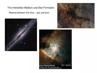

Interstellar Medium and Star Formation
E N D
Presentation Transcript
Interstellar Medium and Star Formation Astronomy G9001 Prof. Mordecai-Mark Mac Low
Dust Excess Mass Visual Nebulae Emission lines Continuum light Polarization Optical Absorption Lines HI lines, & radio continuum UV Absorption lines X-ray emission Molecular line emission IR emission Gamma Rays Historical Overview of Observations
Following Li & Greenberg 2002, astro-ph/0204392 Dust • Naked eye observations of dust clouds • Holes in the heavens (Herschel 1785) vs obscuring bodies (Ranyard 1894, Barnard 1919) • Partial obscuration of continuous nebulae • Smooth dimming of star fields • Shapley-Curtis debate 1920 • Shapley saw no obscuration in globulars: but they were out of plane! • Does obscuration contribute to distance scale?
Reddening • Extinction was known since 1847 (though not taken seriously in Galaxy models) • Reddening discovered by Trumpler (1930) • Wavelength dependence established obscuration as due to small particles • Reddening proportional to NH • Extremely high NH measurable in IR against background star field: NICE (Lada et al. 1994, Cambrésy et al. 2002).
Excess Mass • Vertical stellar motions allow measurement of non-stellar disk mass • Excess density of 6 x 10-24 g cm-3 found by Oort (1932) • We now know that this is a combination of ISM and dark matter. • Similar methods still used to measure dark matter density.
Visual Nebulae • Nebulae first thought to be stellar • Spectroscopy revealed emission lines from planetary nebulae, establishing their gaseous nature (Huggins 1864) • Reflection nebulae distinguished from emission nebulae by continuous spectrum, reddening of internal stars • Measurements of Doppler shifts in emission lines revealed supersonic turbulent motions in Orion emission nebula (von Weizsäcker 1951, von Hoerner 1955, Münch 1958).
Polarization • General linear polarization of starlight by ISM discovered by Hill (1949) and Hiltner (1949). • Alignment of dust in magnetic field (tho mechanism remains debated) • Revealed large scale field of galaxy • Radio polarization of synchrotron shows field in external galaxies as well • At high extinctions (high densities), IR emission polarization fails to trace field (Goodman et al. 1995)
Optical Absorption Lines • Ca II H & K lines have different dynamics from stellar lines in binaries (Hartmann 1904) • Na I D lines behave similarly (Heger) • Now used to trace extent of warm neutral gas • Reveals extent of local bubble (Frisch & York 1983, Paresce 1984, Sfeir et al 99) • Lines spread over 10 km/s, although individual components only 1-2 km/s wide • Interpreted as clouds in relative motion • Reinterpretation in terms of continuous turbulence?
HI lines • HI fine structure line at 21 cm (Ewen & Purcell 1951) reveals cold neutral gas (300 K) • Pressure balance requires 104 K intercloud medium (Field, Goldsmith, Habing 1969) • Large scale surveys show • Supershells and “worms” (Heiles 1984) • Vertical distribution of neutral gas (Lockman, Hobbes, & Shull 1986) • Distribution of column densities shows power-law spectrum suggestive of turbulence (Green 1993)
Radio Continuum • First detected by Reber (1940): Nonthermal • Explanation as synchrotron radiation by Ginzburg • Distinction between thermal (HII regions) and non-thermal (relativistic pcles in B) • Traces ionized gas throughout Milky Way • Evidence for B fields and cosmic rays in external galaxies
UV Absorption Lines • Copernicus finds OVI interstellar absorption lines (1032,1038 Å) towards hot stars • Photoionization unimportant in FUV • Collisional ionization from 105 K gas, but this gas cools quickly, so must be in an interface to hotter gas • First evidence for 106 K gas in ISM
X-ray emission • Confirms presence of hot gas in ISM • Diffuse soft X-ray background (1/4 keV) anticorrelates with NHI: Local Bubble (McCammon et al. 1983, Snowden et al. 1990) • Detection of SNRs, superbubbles • X-ray shadows of cold clouds show contribution from hot halo (Burrows & Mendenhall 1991, Snowden et al. 1991)
Molecular line emission • Substantial additional mass discovered with detection of molecular lines from dense gas • Millimeter wavelengths for rotational, vibrational lines from heterogeneous molecules • NH2 and H2O first found (Cheung et al. 1968, Knowles et al. 1969) then CO (Penzias et al. 1970), used to trace H2 • Superthermal linewidths revealed (Zuckerman & Palmer 1974) showing hypersonic random motions • Map of Galactic CO from roof of Pupin (Thaddeus & Dame 1985)
IR emission • Only with satellite telescopes such as IRAS was IR emission from cold dust in the ISM detectable: the “infrared cirrus” • IR penetrates dust better than visible, so it allows observation of star formation in dense regions
Gamma Rays • Gamma ray emission from Galactic plane first detected with OSO 3 and with a balloon (Kraushaar et al. 1972, Fichtel et al. 1972) • Confirmed by SAS 2 and COS B at 70 Mev. • CR interactions with gas and photons: • Electron bremsstrahlung • Inverse Compton scattering • Pion production • Independent estimate of mass in molecular clouds
Changing Perceptions of the ISM • Densest regions detected first • Modeled as uniform “clouds” • Actually continuous spectrum of ρ, T, P. • Detection of motion showed dynamics • Combined with early analytic turbulence models • Success of turbulent picture limited then • Analytic tractability favored static equilibrium models (or pseudo-equilibrium) • Focus on heating/cooling, thermal phase transitions • New computational methods now bringing effects of turbulence back into focus
Structure of Course • Lectures, Discussion, Technical • Exercises • Class Project • Grading • Exercises (30%) • Participation (20%) • Project (50%)
Project Schedule • Feb 24: Written proposal describing work to be done (1-3 pp.). I’ll provide feedback on practicality and interest. • Mar 10: Oral presentation of final project proposals to class. • Apr 7: Proof-of-concept results in written report (2-4 pp., including figures) • Apr 28: Oral presentation of projects to class in conference format (10-15 minute talks) • May 5: Project reports due
Hydro Concepts • Solving equations of continuum hydrodynamics (derived as velocity moments of Boltzmann equation, closed by equation of state for pressure)
Following Numerical Recipes Discretization • Consider a simple flux-conservative advection equation: • This can be discretized on a grid of points in time and space
t Discretization of Derivatives • The simplest way to discretize the derivatives is just FTCS: • But, it doesn’t work! x
The difference equation is Suppose we assume If |ξ(k)| > 1, then ξn grows with n exponentially! Dividing by ξneikjΔx, and rearranging |ξ(k)| > 1 for some k, so this scheme is unstable Von Neumann stability analysis
Stability (cont.) • This instability can be fixed using a Lax scheme: ρjn->0.5(ρj+1n+ ρj-1n) in the time derivative, so that • Now, if we do the same stability analysis, we find
Courant condition • The requirement that is fundamental to explicit finite difference schemes. • Signals moving with velocity v should not traverse more than one cell Δx in time Δt. • Why is Lax scheme stable?
Numerical Viscosity • Suppose we take the Lax scheme and rewrite it in the form of FTCS + remainder This is just the finite difference representation of a diffusion term like a viscosity.
ZEUS • Program to solve hydro (and MHD) equations (Stone & Norman 1992, ApJSupp) • Details of numerical methods next time: • Second-order discretization • Eulerian moving grid • Artificial viscosity to resolve shocks • Conservative advection formulation
ZEUS organization • Operator splitting (Strang 1968): • Separate different terms in hydro equations • Source, advection, viscous terms each computed in substep:
ZEUS flowchart • Timestep determined by Courant criterion at each cycle
ZEUS grid • Staggered grid to allow easy second-order differencing of velocities • Grid naming scheme…
Boundaries • “Ghost” zones allow specification of boundary values • Reflecting • Outflow • Periodic • Inflow
Version Control • Homegrown preprocessor EDITOR • Clone of 70’s commercial HISTORN • Similar to cpp with extra functions • Modifies code two ways • Define values for macros and set variables • Include or delete lines • A few commands • *dk - deck, define a section of code • *cd - common deck, common block for later use • *ixx - include the following at line xx • *dxx[,yy]- delete from lines xx to yy, and substitute following code • *if def,VAR to *endif - only include code if VAR defined
File Structure • Baroque, to allow “automatic” installation • From the top: • zcomp, sets system variables for local system • zeus34.s compilation script for ZEUS, EDITOR • zeus34, source code with EDITOR commands • zeus34.n, numbered version (next time) • Setup block (next time) generates • inzeus, runtime parameters • zeus34.mac, sets compilation switches (macros) • chgz34, makes changes to code
ZEUS installation • Copy ~mordecai/z3_template • Run zcomp, wait for prompt. (First time takes longer) • View parameters, accept defaults, wait for compile to finish • Make an execution directory (mkdir exe) • Copy xzeus34, inzeus into exe • Run xzeus34. Progress can be tracked by typing n
ZEUS output • To view output use IDL to read HDF files
Assignments • For next class read for discussion: • Ferrière, 2002, Rev Mod Phys, 73, 1031-1066 • Begin reading • Stone & Norman, 1992, ApJ Supp, 80, 753-790 (I will cover more from this paper next time) • Complete Exercise 1 • Install ZEUS, begin reading manual, readme files • Begin learning IDL • Review FORTRAN77 if not familiar