Buffers
Buffers. Buffers minimize memory delays caused by variation in throughput between the pipeline and memory Two types of buffer design criteria Maximum rate for units that have high request rates The buffer is sized to mask the service latency Generally read buffers that you want to keep full

Buffers
E N D
Presentation Transcript
Buffers • Buffers minimize memory delays caused by variation in throughput between the pipeline and memory • Two types of buffer design criteria • Maximum rate for units that have high request rates • The buffer is sized to mask the service latency • Generally read buffers that you want to keep full • Mean rate buffers for units that have a lower expected request rate • The buffer design is sized to minimize the probability of overflowing • Generally, write buffers that you want not to be full
Maximum-Rate Buffer Design • Buffer is sized to avoid “runout”. In this case the processor stalls while the buffer is empty awaiting service. • Need buffer input rate > buffer output rate • Then size to cover latency at maximum demand • For I buffer, the buffer size (BF) should beBF = 1+[(Instrs decoded/~)*(IF latency in~)]/Instrs/IF
Maximum-Rate Buffer Example Assumptions: Decode consumes max 1 inst/clock Icache supplies 2 inst/clock bandwidth at 6 clocks latency
Mean-Rate Buffer Design • Buffer is sized to avoid “overflow”. In this case the processor stalls while the buffer is awaiting service to free an entry. • Need buffer input rate < buffer output rate • Then size to reduce frequency of overflow to acceptably low level with respect to overall performance
Mean-Rate Buffer Design • Use inequalities from statistics to target buffer size • For infinite buffer, assume distribution of buffer occupancy is q and mean occupancy is Q • Using Markov’s inequality for buffer of size BF Prob of overflow = p(q >= BF) <= Q/BF • Using Chebyshev’s inequality for buffer of size BF Prob of overflow = p(q >= BF) <= 2/(BF- Q)2 • for a given probability of overflow (p), conservatively select BF BF = min(Q/p,Q +/ p) • Analyze design carefully to pick correct BF that causes overflow/stall
Mean-Rate Buffer Example Reads MemoryReferencesfromPipeline DataCache StoreBuffer Writes Assumptions: store rate = 0.15 inst/cycle store latency to data cache = 2 clocks 2 = 0.3 BF = 2
Cache • Design Target Miss Ratio (DTMR) • DTMR is the design target miss rate assuming fully associative, unified cache with LRU replacement • Includes compulsory and capacity misses for user-only traces
Cache • Apply adjustments to DTMR • Associativity • split Instruction/Data • Write Policy: Write-Through (WT) or Copy Back (CB) • Write Allocate (WA) vs. No Write-Allocate (NWA) • Replacement Policy • OS, multiprogramming, and I/O effects
Target Miss Rate Trend • Target Miss Rates tend to increase over time • programming environments become more complex • application functionality increases • problem size grows • memory capacity increases
System Effects • Operating System • Multiprogramming • Q = no. instructions between task switches • Cold-Start vs. Warm-Start • Cold-Start • short transactions are created frequently and run quickly to completion • Warm-Start • long processes are executed in time slices
Multi-Level Caches • Very useful for matching processor to memory • Generally 2-level • For microprocessors, L1 on-chip at frequency of pipeline and L2 off-chip at slower latency and bandwidth
Multi-Level Caches • Analysis by (statistical) inclusion • If a L2 cache is greater than four times the size of the L1 cache then we assume statistically that the contents of L1 lies in L2 • Relevant L2 Miss Rates • Local Miss Rate: No. L2 misses / No. L2 references • Global Miss Rate: No. misses / No. processor references • Solo Miss Rate: No. misses without L1 / No. processor references • Inclusion => Solo miss rate = Global miss rate • Miss penalty calculation • L1 miss rate x (miss in L1, hit in L2 penalty) plus • L2 miss rate x ( miss in L1, miss in L2 penalty - L1 to L2 penalty)
Multi-Level Cache Example Memory L1 L2 Miss Rate 4% 1% Delays: Miss in L1, Hit in L2 2~ Miss in L1, Miss in L2 7~ Cpi loss due to L1 is 1.5 refr/instr x 0.04 x 2~/miss = 0.12 Cpi loss due to L2 is 1.5 refr/instr x 0.01 x (7-2) ~/miss = 0.075
Logical Inclusion • In multiprocessors it is important to know exactly that the L1 cache does NOT contain a line by determining that the L2 cache does not have this line. • Reduces latency and bandwidth for snooping • For this purpose we need to insure that all the contents of L1 are always in L2 • We call this property Logical Inclusion
Logical Inclusion • Techniques • Control Cache size, organization, policies • No. L2 sets >= No. L1 sets • L2 set size >= L1 set size • Compatible replacement algorithms • But this is highly restrictive and difficult to guarantee • Back-invalidation • Whenever a line is replaced or invalidated in the L2, ensure that it is not present in L1 or it is evicted from L1
Outline: Memory and Queuing Models • Physical Memory • Memory Technology • Simple Memory Performance Models • Hellerman • Strecker
Outline: Memory and Queuing Models • Basic Queuing Models • Terminology • Approximations • Key Results • Application of Queuing Models to Memory Performance • Interleaved memory • Cache • Bus
Memory • Processors are increasingly limited by memory and not processor organization or cycle time. • Memory is characterized by 3 parameters • size • access time (latency) • cycle time (bandwidth)
Achieved vs. Offered Bandwidth Offered Request Rate: • Rate that processor(s) would make requests if memory had unlimited bandwidth and no contention
DRAM Technology (text section 6.2) • DRAM cell • Capacitor used to store charge for 0/1 state • Transistor used to switch capacitor to bit line • Charge decays over time => refresh required
DRAM Technology (text section 6.2) • DRAM array • Stores 2n bits in a square array • 2n/2 row lines connect to Tx gates • 2n/2 column bit lines with sense amp • DRAM chip • Row and column addresses muxed • Row/Column Strobes for timing
Technology and Market Trends • Market Trends • Demand for minimum/incremental memory growing only ~30% per year for PCs • Bandwidth requirements growing rapidly • driven by multimedia (esp. video and graphics) => caches do not help • Fill Frequency captures this trend • Rate at which it is possible to read/write all of memory • Bandwidth[MB/sec] / Memory Size [MB] • Example PC: 500 MB/sec for 32MB => 15.6 Hz fill frequency
Technology and Market Trends • Technology Trends • Capacity increases 60% per year • Access time decreases 7% per year • Cost/bit decreases 26% per year As DRAM Density Increases, Need More Bandwidth and Fewer Memory Chips With Few Pins
Techniques to Increase DRAM Bandwidth • Fast Paged Mode • Synchronous DRAM • Rambus (RDRAM)
Fast Page Mode (FPM) • Page Mode => Save most recently accessed row (“page”) • Only need column row and CAS to access within the page • Fast Page Mode • Counter built into RAM for sequential accesses • Only need CAS for sequential accesses • With Extended Data-Out (EDO) can cycle at 33-50 MHz
Synchronous DRAM (SDRAM) • Clocked (Synchronous) interface enables pipelined access • Internally implemented with dual banks for higher throughput • Clock rates of 100-150 MHz possible • Dual Data Rate (DDR SDRAMS) • proposal to transfer 2 data bits per clock • target 200 Mb/s at 100 MHz • technically feasible, but demanding system requirements
RAMBus DRAM (RDRAM) • Channel interface bus replaces row/column address • 9 data signals, 4 clock and control signals • Protocol for transferring address and data bursts • Clock frequency currently 266 MHz with 533 MB/s • Up to 32 RDRAMs per channel • Die area ~10% overhead for 16Mb DRAM • SLDRAM is open standard with similar technology From IEEE Micro 11/97
RAMBus DRAM (RDRAM) • Channel interface bus replaces row/column address • 9 data signals, 4 clock and control signals • Protocol for transferring address and data bursts • Clock frequency currently 266 MHz with 533 MB/s • Up to 32 RDRAMs per channel • Die area ~10% overhead for 16Mb DRAM
RAMBus DRAM (RDRAM) • SLDRAM is open standard with similar technology From IEEE Micro 11/97
Memory Module • The module consists of the DRAM chips that make up the physical memory word. In addition to the DRAM chips there are memory controller, timing and bus driver chips. • If the DRAM is organized 2n words xb bits and the memory has p bits/ physical word then the module has p/b DRAM chips.
Memory Module • The module has 2n words xp bits • Parity or Error-Correction Code (ECC) generally required for error detection and availability • Text section 6.2.2 describes code forSingle-Error Correction, Double-Error Detection (SECDED) • Requires ~ extra log2(p) + 1 bits
Memory system • Consists of multiple modules that are interleaved by low order or high order address bits (or both). • Low order interleaving improves memory BW • High-order interleaving improves availability
Processor memory model • Assume that n processors each make one request each Tc to one of m memory modules. B(n,m) is number of successes. • Tc is the memory cycle time, Ta is the memory access time. • To the memory one processor making n request per Tc behaves as n processors making 1 request per Tc.
Basic terms • B = B(m,n) or B(m) is number of requests that succeed each Tc. It is the bandwidth normalized to Tc. • Ts is a more generalized term for service time. Tc = Ts. Used in I/O models. • BW is the achieved bandwidth in requests serviced per second. BW = B / Ts = B(m,n) /Tc
Modeling and Evaluation Methodology • Identify relevant physical parameters • for memory: word size, module size, no. modules, Tc, Ta • Find the offered Bandwidth • n/Tc • Find the bottleneck • performance limited by most restrictive service point
Modeling and Evaluation Methodology • Determine the type of reference pattern • sequential, stride, random • Select an appropriate model • Use the simplest possible • Evaluate the achieved bandwidth • B(m,n) for memory
Models for computing B(m,n); text 6.3 • Hellerman’s..... B(m) = m • Limited, unrealistic model • single processor generates random references in-order until bank conflict • Only historical interest: “the square-root rule” • Strecker’s (the null binomial) • Queue models • open • closed • mixed
Strecker’s model • Model description • Each processor generates 1 reference per cycle • Requests random and uniformly distributed across modules • Any busy module serves 1 request • All unserviced requests are dropped each cycle • There are no queues • B(m,n) = m[1 - (1 - 1/m)n]
tw ts t Queuing Models, text 6.4 • Arrival process • Server • Occupancy/Utilization • Time • Number of items Art of Computer Systems Performance Analysis, Raj Jain, Fig. 30.2
Key Model Characteristics • Queuing Models characterized by 3-tuple • arrival distribution • service time distribution • No. Servers • E.g., G/G/1 for general arrival and service distribution • Arrival distributions we will use • MB, the Binomial distribution • M, the Poisson distribution • inter-arrival times are exponentially distributed • limiting case of the Binomial
Key Model Characteristics • Service distributions we will use • M, exponential service time • D, deterministic service time (constant) • We will generally be looking for mean values • time in system, utilization
Binomial arrivals, text 6.4.1 • Description • n items enter system with has m modules • requests are randomly distributed across modules with equal probability 1/m(Bernoulli trial) • Probability that k out of n requests are to a specific module • Pn(k) = C(kn)(p)k(1-p)n-k • 1 -Pn(0) = B(m,n) from Strecker’s model
Poisson distribution, text 6.4.1 • Assume n and m very large, then p is small but np, the expected no. of arrivals at the server during T, is finite. • np/T and p = T/n • Then P(k) = [(T)k/k!] e- T
Queuing Properties, text 6.4.5 • No. itemsitems in system = items in queue + items in service • Mean valuesN = Q + r • Little’s result: N = T and Q = Tw • Service Distributions • Coefficient of variation = c = • For exponential distribution c = 1 • For deterministic (constant) distribution c = 0
Pollaczek-Khinchin (P-K) Theorem • For M/G/1Mean waiting time Tw = (1/)[ 2(1+c2)/2(1-)]Mean items in queue Q = Tw = 2(1+c2)/2(1-) • Cases of interest • For M/M/1, c2 =1Tw = (1/)[ 2/ (1-)]Q = 2/(1-) • For M/D/1, c2 = 0Tw = (1/)[ 2/ 2(1-)]Q = 2/2(1-) • For MB/D/1, c2 =0Define p =/m where is the prob. that a source makes a requestTw = (1/)[ (2-p)/2(1-)]Q = (2-p)/2(1-)
Open vs Closed queues, text 6.5 • Open Queue Models • Arrival process is independent of queue size • Processor not slowed (or otherwise affected ) by contention • Queue size is unbounded • Closed Queue Models • Arrival rate slows down as queue grows • If n items are offered and the system initially accepts only B, then the queue size Q = n-B
Open vs Closed queues, text 6.5 • Mixed Queue Models • Buffers allow arrival rate to continue without slowdown (like open queue) until queue size reaches a threshold, then arrival rate starts slowing down (like closed queue) • Use this later for I/O
Closed Queues, text 6.5.2 • From the P-K theorem for total queue sizeN = a +[ a2(1+c2)/2(1-a)] • N = n/m • n/m per Tc is offered to each module • a is achieved • and Tw =m-1[( - a)/a] • B(m,n) = ma, solving for B(m,n) in asymptotic case • for M/D/1 • a =( + 1) -2 + 1 • B(m,n) = m + n - n2 + m2 • for MB/D/1 • B(m,n) = m+n-1/2 - (m+n - 1/2)2- 2mn