Download
1 / 56
610 likes | 912 Vues
The Real Business Cycle School. Intermediate Macroeconomics ECON-305 Spring 2013 Professor Dalton Boise State University. RBC Macroeconomics. Evolved out of New Classical economics of 1970s Major proponents Edward Prescott (Minnesota) Finn Kydland (Carnegie-Mellon)

E N D
The Real Business Cycle School Intermediate Macroeconomics ECON-305 Spring 2013 Professor Dalton Boise State University
RBC Macroeconomics • Evolved out of New Classical economics of 1970s • Major proponents • Edward Prescott (Minnesota) • Finn Kydland (Carnegie-Mellon) • Charles Plosser (Rochester) • Robert Barro (Harvard)
From New Classical to RBC • The late 1970s and early 1980s was a time of New Classical Dominance • By the early 1980s, however, significant doubts had arisen • “signal-extraction” problem not robust enough to explain business cycles • Evidence supportive of monetary neutrality of announced policy weak • Tobin suggests a “way out” that he does not himself take seriously – random real shocks
From New Classical to RBC Kydland and Prescott take seriously this alternative and develop the foundations of Real Business Cycle Theory – a theory that accounts for cycles wholly by changes in real supply variables. Kydland and Prescott, “Time to Build and Aggregate Fluctuations,” Econometrica (November 1982) Originally viewed as augmenting the New Classical approach
Central Proposition Large random fluctuations in technology produce supply-side shocks to the production function, generating fluctuations in aggregate output and employment as rational individuals respond to the altered structure of relative prices by changing labor (resource) supply and consumption (investment) decisions.
RBC Macroeconomics • Assault on all previous 20th century macroeconomics • Booms are not “good” and recessions are not “bad” • Recessions are not desired by agents in the economy but they are nonetheless unavoidable consequences of changes in constraints agents face
RBC Macroeconomics • Assault on all previous 20th century macroeconomics • Agents react optimally to changes in constraints and the resulting aggregate fluctuations are efficient • Supply, not demand shocks, are key to understanding economic fluctuations
RBC v. New Classical • RBC replaces the impulse mechanism of New Classical economics • “Technology shocks” instead of “monetary surprise” • RBC retains the propagation mechanisms of New Classical economics • Rational expectations and relative prices • New Classical Economics “Mark II”
Reactions of Leading New Classicalists • Lucas • Exclusion of money in RBC a mistake • Viewed as addition to NC models • Later says “monetary shocks just aren’t that important” • Approves of methodology • micro-based models and use of fully-articulated artificial economies to compare real with experimental economics • Business cycles are “minor problem” – shifts focus to Growth economics
Reactions of Leading New Classicalists • Barro • RBC promising • Monetary neutrality of New Classical models a “mistake” • Shifted focus to Growth economics • Defends New Classical Achievements • Equilibrium modeling • Rational expectations • Dynamic policy-making and evaluation
Growth and Cycles Development of RBC and shift of research to Growth represent revival of interest in “supply-side” macroeconomics Continuation of pre-Keynesian lines of business cycle research New technology influences both long-run growth as well as producing short-run displacements (disequilibrium?)
RBC Antecedents • Dennis Robertson • emphasized real forces • Joseph Schumpeter • “Theory of Capitalist Development” • Knut Wicksell • Changes in marginal productivity of capital (impulse mechanism) cause divergence of “natural rate of interest” from “bank loan rate” leading to endogenous monetary creation (propagation mechanism), distorting time structure of production and leading to self-reversing boom
Growth and Cycles For Real Business Cycle Macroeconomics, growth and cycles are inseparably interrelated
History and RBC • Supply shocks of 1970s • Two OPEC oil increases • Apparent failure of Demand-side Keynesian model • Political emphasis of “new supply-side economics” of Reagan Administration • Tax cuts and deregulation • Renewed interest in statistical properties of economic time-series • Seminal work of Nelson and Plosser
Cycles and Random Walks • Conventional Approach • Imagines economy evolving along a growth path reflecting underlying trend • Fluctuations about trend due to demand shocks • Shocks “die out” over time, so economic time-series are “trend-reverting” • Yt = gt(Y0) + b (Y – YT)t-1 + zt
Cycles and Random Walks Y time Yt = gt(Y0) + b (Y – YT)t-1 + zt At time t1, a shock of size z occurs, but it dies out over time and the growth path reverts to the trend Conventional approach consistent with the natural rate hypothesis (unanticipated changes in monetary growth produce temporary deviations from YN)
Cycles and Random Walks Nelson and Plosser, “Trends and Random Walks in Macroeconomic Time Series: Some Evidence and Implications,” Journal of Monetary Economics (September 1982) Most changes in GDP are permanent, with no tendency for Y to revert to former trend GDP follows a random walk process with drift
Cycles and Random Walks • Nelson-Plosser Approach • Value in one period still dependent on previous value of the variable, but shocks (z) change output permanently • Rather than g being underlying growth rate, g is “rate of drift;” b has value of 1 – “unit root” hypothesis • Yt = gt(Y0) + (Y – YT)t-1 + zt
Cycles and Random Walks Y time Yt = gt(Y0) + (Y – YT)t-1 + zt At time t1, a shock of size z occurs and it permanentlychanges the growth path of the economy
Implications of Nelson-Plosser • Observed fluctuations are fluctuations in the trend, not deviations from a trend. • In NC world, permanent changes in GNP growth cannot occur from monetary shocks since money is neutral; therefore main forces causing instability must be realshocks. • If shocks to productivity growth are frequent and random, path of Y follows a random walk that resembles the business cycle. • No distinction between trend and cycle, so theory of growth and fluctuations must be integrated.
Productivity Shocks Unfavorable changes in the physical environment that adversely affect agricultural output Significant changes in price of energy War, political upheaval and labor unrest Government regulations Changes in the quality and quantity of capital and labor; new management techniques; new products; new production techniques =>Technological change
RBC Models: Common Features (1) Representative agent models; agents maximize s.t. constraints (2) Agents form Ratex; signal-extraction problem re permanent v. temporary productivity shocks (3) Continuous market-clearing (4) Exogenous productivity shocks are impulse mechanism for output and employment fluctuations
RBC Models: Common Features (5) Propagation mechanisms vary, include consumption smoothing, “time-to-build,” and intertemporal labor substitution (6) Fluctuations in employment voluntary; labor and leisure highly substitutable over time (7) Money is neutral (8) No distinction between SR and LR
Changes from New Classicalism Impulse factor – productivity shocks replace monetary shocks Abandon price level/relative price misperception emphasis Abandon long run/short run distinction
RBC: Model Structure • Production Function • Yt = At F(Kt, Lt) • Technology Evolution Parameter • At+1 = þAt + єt+1 0 < þ < 1 • Representative Agent Utility Function • Ut = f(Ct, Let) • Resource Constraints • Ct + It ≤ Yt; Lt + Let ≤ 1 • Capital Stock Accumulation Equation • Kt+1 = (1-∂) Kt + It
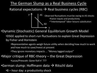
Technology Shocks and Employment • Technology shocks change A, shifting the production function upward; the demand for labor curve will also shift upward. • Increased labor demand will increase the real wage and employment. • How much? Depends on supply elasticity! • If labor supply is inelastic? • If labor supply is elastic?
Technology Shocks and Employment Stylized facts of Business Cycles indicate small procyclical variations in real wage are associated with large procyclical variations in employment Is labor supply highly elastic or inelastic with respect to real wage? What does that indicate about the intertemporal substitution of labor for leisure?
RBC and Lucas-Rapping ASH • Lucas-Rapping: in making labor-supply decisions, workers consider future and current C and Le • Substitution and income effects of changed real wage • Temporary v. permanent changes in real wages
RBC and Lucas-Rapping ASH • RBC • temporary technology shocks will lead to temporary changes in real wages; no income effect and large supply response • Permanent technology shocks will lead to permanent changes in real wages; large income effect and small supply response
Labor Supply and Interest Rates • Change in the real interest rate affects labor supply by altering relative price of income earned today v. future • Ls = Ls(W/P, r) • Intertemporal price-ratio (1+r) (W/Pt) (W/Pt+1) • Increase in r increases labor supply; reduction in r reduces labor supply
RBC AD and AS r RAS LM/P IS (RAD) Y An IS-LM model conforming to Ratex, Continuous Market Clearing, and Full-information Ms Output and employment due to real forces; RAS determined by production function and labor supply Tech improvement shifts RAS to right and LM/P adjusts so full employment exists Problem with model: Labor supply not dependent on r
RBC AD and AS r RAS re RAD Y Ye If labor supply is dependent on r, an increase in r increases labor supply and increases output The RAS curve is positively sloped
Characteristics of Model Model entirely real (M and P have no impact on Y or L) No LR-SR distinction RAS traces out labor market equilibria r equilibrates goods market Shifts in RAS lead to variations in Y and L Temporary variations in RAD can cause Y and L variations
Technology Shock: RAD-RAS Y Y Y = Y Y* b Y b a a Y SL2 (r2) w r SL1 (r1) RAS1 w2 b RAS2 r1 a w1 DL2 r2 b a RAD DL1 L1 L2 L Y1 Y2 Y Begin in equilibrium. Labor market clears at real wage w1 for given production function Y. At current r1, RAS and RAD clear at Y1. Favorable productivity shock increases A and production function increases to Y*. RAS increases, driving down the interest rate. The lower interest rate lowers the supply of labor and favorable productivity shock increases labor demand. Labor market equilibrium moves to b, employment increases and output increases at the lower interest rate.
Expenditure Shock: RAD-RAS Y Y Y = Y b Y b a a Y SL1 (r1) w r RAS SL2 (r2) r2 b r1 a a w1 w2 b RAD2 DL1 RAD1 L1 L2 L Y1 Y2 Y Begin in equilibrium. Labor market clears at real wage w1 for given production function Y. At current r1, RAS and RAD clear at Y1. Increase in government purchases shifts RAD to the right, increasing the real interest rate. The higher interest rate increases the supply of labor and reduces the real wage rate. Labor market equilibrium moves to b, employment increases and output increases at the higher interest rate.
Temporary v. Permanent Shocks • In the previous model, wealth effects were ignored. • If shocks are permanent, wealth effects can’t be ignored. When permanent shocks occur, induced changes in the real wage also will led to additional changes in RAD. • A change in technology will cause RAS and RAD to move in the same direction. • A positive technology shock that raises RAS raises the real wage, increases real income and increases RAD. • A change in expenditures will moderate the change in RAD. • An increase in government purchases that reduces the real wage reduces real income and decreases RAD.
Temporary v. Permanent Shocks r RAS RAS2 re r2 RAD2 RAD Ye Y2 Y A positive technology shock increases RAS to RAS2. If the shock is temporary, the wealth effect is small and RAD increases by a small amount. The real interest rate falls as higher output is achieved. This does not change the prediction of the model which ignores wealth effects.
Temporary v. Permanent Shocks r RAS RAS2 re RAD2 RAD Ye Y2 Y A positive technology shock increases RAS to RAS2. If the shock is permanent, the wealth effect on expenditures will be large and increase RAD by roughly the same amount as the increase in Y. Out put increases but the interest rate remains approximately the same. This prediction of the model is different than that which ignores wealth effects.
“Testing” RBC Models • Kydland and Prescott were first to show that RBC models could generate time-series data that possessed statistical properties similar to actual US business fluctuations. • RBC theorists generally have not attempted to provide models capable of econometric testing. • Instead, RBC theorists have developed the method of calibration to test their models.
Calibration Method (1) Construct RBC equilibrium model (2) Provide specific functional forms (3) Calibrate the model - simulate random shocks with computer generated random numbers (4) Trace out key macroeconomic variables from exercise and compare with actual time-series
Calibration Method • Such exercises are able to mimic the actual economy with respect to important time-series data and replicate the stylized facts of business fluctuations • Problem: How to choose between competing models? No criteria equivalent to significance testing in econometrics to answer such a question.
RBC and Money • Accepted stylized fact: Positive correlation between money and output. • Generally accepted (Friedman and Schwartz) by Keynesians, Monetarists and New Classicalists that changes in monetary growth cause changes in real output growth. • In RBC models, money is “super” neutral. How do RBC models account for the accepted stylized fact?
RBC and Money • Caveat: Positive correlation between money and output may indicate that money responds to output. • But then why does it look like monetary growth comes before output growth? • Expectations of future output growth may lead to increases in money demand that increase the quantity of money supplied. • Bank money (demand deposits) is endogenous; bank money can be produced faster than real output. • Money supply changes before output but output changes cause money supply changes.
RBC and Money • RBC theorists divided into two camps • Kydland and Prescott, “Business Cycles: Real Facts and the Monetary Myth,” FRB Minneapolis Quarterly Review (Spring 1990) • Denial of stylized fact that money leads the cycle • Plosser, “Understanding Real Business Cycles,” Journal of Economic Perspectives (Summer 1989) • Role of money remains an “open question”
Measuring Technology Shocks • How does one measure technological progress? • “Solow residual” • That part of ∆Y that can’t be explained by ∆K or ∆L • Y = A F (K, L) • Y = A KβL1-βwhere 0 < β < 1 • ∆Y/Y = ∆A/A + β ∆K/K + (1- β) ∆L/L • ∆A/A = ∆Y/Y – [β ∆K/K + (1- β) ∆L/L]
Measuring Technology Shocks • Prescott (“Theory Ahead of Business Cycle Measurement”) suggested (∆A/A) is a random walk with drift plus serially uncorrelated error • Plosser (“Understanding Real Business Cycles”) uses (∆A/A) and (∆Y/Y) to show that aggregate fluctuations in Y are mainly due to fluctuations in technology
The Stylized Facts • RBC literature led to a renewed effort to discover and measure the stylized facts of business fluctuations • Forced a re-evaluation of existing theories in light of the new data • Central controversies over • Real wages • Price level
Real Wages and Business Cycles • Are real wages pro-cyclical or counter-cyclical? • Orthodox Keynesianism and Orthodox Monetarism • Real wages are counter-cyclical • Changes in AD with sticky or lagging wages (due to adaptive expectations) • RBC • Real wages are strongly pro-cyclical • Changes in technology shift production function and change the demand for labor • Empirics • Real wages are slightly pro-cyclical • Problem: procyclical wages require elastic labor supply to produce observed variations in employment and output, but micro data does not support notion of elastic labor supply
Price Level and Business Cycles • Is the price level pro-cyclical or counter-cyclical? • Orthodox Keynesianism, Monetarism, New Classical • Price level and inflation are pro-cyclical • RBC • Evidence from entire 1954-89 period is that price level and inflation are counter-cyclical • Empirics and Impulse Mechanisms • Impulse determines behavior of price level and inflation • Supply-side changes lead to counter-cyclical prices • Demand-side changes lead to pro-cyclical prices