High-Frequency Trading Analysis: Micro-Vertexing in the HFT Era
220 likes | 298 Vues
Explore the implementation and significance of micro-vertexing in high-frequency trading analysis, focusing on decay length, D0 particle characteristics, tracking techniques, and PID considerations. Understand the importance of full track information, covariance matrices, and secondary vertex fit methods in multivariate analysis to optimize results in the HFT landscape.

High-Frequency Trading Analysis: Micro-Vertexing in the HFT Era
E N D
Presentation Transcript
D0 analysis in HFT era with (mVertex) code LBL May 12, 2010 BNL: Y. Fisyak, V. Perevoztchikov [A. Kisel (guest)] Kent:J. Bouchet, J. Joseph, S. Margetis, J. Vanfossen
Why micro-Vertexing ? • What is it? How is it implemented? • Recent work • What is next? OUTLINE
counts D0->K+pi ~1 c Decay Length in X-Y plane cm • Very short lived particles • For a realistic D0 distribution at mid-rapidity (<pT>~1 GeV/c) the average decay length is 60-70 microns Why micro-Vertexing ? • Used <pt>~1GeV • 1 GeV/ =0 D0 has • Un-boost in Collider ! • Mean R-f value ~ 70 mm
Hard (fixed value) cuts are not optimal • Need to use momentum depended/correlated cuts otherwise one strongly biases result • One example is pointing (DCA) resolution • Pointing (DCA) info is at least as important in mVertexing as dE/dx to PID people !! SVT+SSD dcaXY vs 1/p 10
Need to use full track info • Full covariance/error matrix • Need to have track info inside beam pipe • So that helix hypothesis is exact solution • So that error matrix is optimal w/out new-material terms • This should be the way to do this analysis; it is in HEP • This should be the way of the (HFT) future One other important step in the multi-dimensional analysis of cut variables as done, e.g. by XM Sun and Yifei
TRACKING (‘OLD’) • Find Global Tracks -> Save info @ first measured hit • Find Vertex • Fit/Find Primary Tracks • TRACKING (‘NEW’) • Find Global Tracks • Move them through all material to beam pipe center (x,y)=(0,0) • Save FULL track/error info -> DcaGeometry • Use THIS for secondary vertex searches • This info is in MuDst starting with Run-7 Au+Au data • For optimal silicon analysis • We can always retrofit Cu+Cu What is it? How is it implemented ?
DcaGeometry Pt_GL track trajectory (first hit) . (circle center) Pt @ DCA .(0,0) . Event DCA x Beam Pipe SVT1,2 R-F plane
DcaGeometry • PT grows as we move backwards • Errors/cov-terms change too • No-huge but finite effect +SVT 3 2 1 TPC+SSD TPC only
Caution: dEdx introduces x-talk All Possible Accepted
Pure D0(Monte Carlo sample) With a cut on the charge of the daughter Tracks, QGlKaon<0&&QGlPion>0 QGlKaon<0&&QGlPion>0 QGlKaon>0&&QGlPion<0 QGlKaon<0&&QGlPion>0 QGlKaon>0&&QGlPion<0&& 0.3<Cos(θ*)<0.7 Mass due to misidentification of daughter Tracks • PID mis-identification makes a D0->D0bar and vice-versa • This introduces a pseudo-enhancement in signal region inv.mass • Wider mass due to wrong kinematics • Needs to be evaluated via Embedding
Kaon decay angle In cm frame • Previous studies showed that abs(cos-theta*)<0.6 cuts most background • It also avoids kinematical edges (soft kaon/pion)
Secondary vertex fit methods used • Linear fitabandoned. • Helix swimming to DCA of the two track helices (V0-like) using the global track parameters to reconstruct helices (StPhysicalHelix) not saved . • Helix swimming to DCA of the two track helices (V0-like) using the parameters from StDcaGeometry: save full track information (covariance matrix) inside the vacuum (center of beam pipe). • Full D0/Helix Fit (TCFIT) with vertex constraint and full errors • Also a full Kalman D0-fit was tried but not significant gains in time etc • The combined info from points 3, 4 will allow momentum dependent cut using the full track information. • Least square fit of the decay vertex. In 2 body decay, combination of 2 tracks + addition of constraint(s) to impose ‘external knowledge’ of a physic process and therefore force the fit to conform to physical principles. • The Kalman fitter machinery allows the knowledge with high precision of tracks near the primary vertex (by taking into account the MCS due to the silicon layers).
Long-ctau D0 evaluation • Each plot shows the correlation of the secondary vertex position from GEANT (y-axis) with 1 of the 3 methods investigated : TCFIT,global helix and DCA geometry helix (x-axis) for its 3 components. TCFIT GEANT DCA X Y Z J.Vanfossen RECO
‘normal’ c D0 evaluation • TCFit does a bit better job than either helix swimming method. • The scatter along the x axis of the swimming methods can be attributed to low pt D0’s and daughter tracks that are close to being parallel or anti parallel. X Y Z J.Vanfossen
Resolution plots 230µm 230µm 190µm • TFCIT makes a better job in terms of resolution 270µm 260µm 250µm 270µm 260µm 250µm J.Vanfossen
Real Data • Run over run 7 data productionMinBias. • Sample is ~35 Million events/ ~55 vertices • QA plots done day by day : • http://drupal.star.bnl.gov/STAR/blog/bouchet/2010/feb/24/full-production-minbias-run7 • Cuts (see next slide) chosen to speed the code.
Cuts used (real data) • EVENT level • triggerId : 200001, 200003, 200013 • Primary vertex position along the beam axis : |zvertex| < 10 cm • Resolution of the primary vertex position along the beam axis: |zvertex|< 200µm • TRACKS level • Number of hits in the vertex detectors :SiliconHits>2 (tracks with sufficient DCA resolution) • Momentum of tracks p >.5GeV/c • Number of fitted TPC hits > 20 • Pseudo-rapidity :||<1(SSD acceptance) • dEdxTrackLength>40 cm • DCA to Primary vertex (transverse) DCAxy< .1 cm • DECAY FIT level • Probability of fit >0.1 && |sLength|<.1cm • Particle identification : ndEdx :|nK|<2, |nπ|<2
D0 signal in 2007 Production mbias • Cuts(offline): • 50µm< decaylength<400µm • trackDca<200 µm • dcaD0toPV<300µm • pTkaon>0.7GeV/c • pTpion>0.7GeV/c • Plot as a function of gRefMult J.Joseph
50<gRefMult S/N ~ 5.7 J.Joseph
Outlook • D0-vertex code has been used in data analysis and it is debugged • Can be used to analyze HFT data (see next talk) • The use of Kalman vertex fitter has the advantage of easy upgrade to more than 2 daughter particles. • Cut-set selection, optimization and apple-2-apple comparisons is next
Constrained vertex fit • 2 = ∑(yi0 - yi(x*))TV-1(yi0 - yi(x*)) + F where : • x* : secondary vertex position • yi0 : track parameter of the original fit • y : track parameter after refit with knowledge of the secondary vertex • V : covariance matrix of the track parameter • i : sum over tracks • F : constraint f • f : physical process to satisfy K- π+ 3d path length from primary vertex to decay particle vertex • The constraint(s) is(are) added to the total 2 via Lagrange multiplier • The minimum of 2 is then calculated with respect to the fit parameters x and with respect to because the condition ∂2/∂ =0 required for the minimum correspond the the constraint equation f