Download
1 / 46
460 likes | 614 Vues
A particle one decay:. But the integral is not Lorentz invariant!. We make it more complicated by allowing an indefinite p 0 and then fixing it:. But in this form, we can be sure it is Lorentz invariant!. We can perform the p 0 integration to recover the 3 space form.

E N D
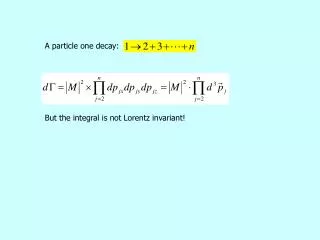
A particle one decay: But the integral is not Lorentz invariant!
We make it more complicated by allowing an indefinite p0 and then fixing it: But in this form, we can be sure it is Lorentz invariant! We can perform the p0 integration to recover the 3 space form. This is Lorentz invariant.
But M2 is still not Lorentz invariant. Γ transforms like 1/t1. t1 transforms like E1. Now we can be sure M2 is Lorentz invariant. It’s called Feynman Amplitude.
Now we apply this to pion two photon decay. Choose the rest frame of pion:
Two body scattering: as you would expected If we consider only Lorentz transformation along the 1-2 colliding axis, the cross section is invariant! But we do want to pull out a Lorentz invariant factor that reflects the inverse flux that must appear in cross section:
Feynman Rules To evaluate the Lorentz Invariant Feynman Amplitude M Components of Feynman Diagrams External Lines Particle Content (their masses and spins) Internal Lines propogator Vertex Interactions
For a toy ABC model Three scalar particle with masses mA, mB ,mC Factors 1 External Lines Internal Lines C Vertex -ig A B
Draw all diagrams with the appropriate external lines Integrate over all internal momenta Take out an overall momentum conservation. That’s it! It’s so simple.
Each extra vertex carries an extra factor of –ig, which is small. Consider first the diagrams with the fewest number of vertices.
Scattering To the leading order, there could be more than one diagrams! In the diagrams, the B lines in some vertices are incoming particle. The striking lesson: Lines in a vertices can be either outgoing or incoming, depending on their p0. p0 for an observed particle is always positive. So this vertex diagram is actually 8 diagrams put together! That’s the simplicity of Feynman diagram.
The momentum conservations can be carried out immediately in the beginning! The result can be written down right away! This page also teaches us an important lesson: After momentum conservation is enforced, the momentum of internal particle c is It does not satisfy momentum mass relation of a particle! The internal particle is not a real particle, it’s virtual.
媒介粒子 γ 交互作用是透過交換媒介粒子來進行 媒介粒子媒介一個交互作用
交互作用不只改變粒子的動量,也可能改變粒子的身分!交互作用不只改變粒子的動量,也可能改變粒子的身分! n p p n
媒介粒子 媒介粒子只有在交互作用進行中存在,如果只觀察物體前後變化,就不會看到它。它幾乎不是一個實在的粒子,而是一個虛粒子。 虛粒子即使不穩定地存在,也會透過它所媒介的交互作用,影響實在的世界 So heavy particles, though decay fast and don’t existent in nature, do matter. (they could be virtual)
It does not satisfy momentum mass relation of a particle! The internal particle is not a real particle, it’s virtual. In a sense, the relation is only for particles when we “see” them! Internal lines are by definition “unseen” or “unobserved”. It’s more like: It’s more a propagation of fields than particles!
Field fluctuation propagation can only proceed forward that is along “time“ from past to future. This diagram is actually a Fourier Transformation into momentum space of the spacetime diagram. The vertices can happen at any spacetime location xμ and the “location” it happens need to be integrated over. After all you do not measure where interactions happen and just like double slit interference you need to sum over all possibilities.
For those amplitude where time 2 is ahead of time 1, propagation is from 2 to 1. For those amplitude where time 1 is ahead of time 2, propagation is from 1 to 2. B B B B 2 1 1 2 C C A A A A is actually the sum of the above two diagrams! Feynman diagram in momentum space is simpler than in space-time!
Lesson 3: In this diagram, particles seem to have certain momenta. According to uncertainty principle, their position uncertainty is infinity! This diagram is only an approximation of more precise treatment using wave packet! You need to “superpose” similar diagrams with slightly uncertain momentum t produce incoming and outgoing wave packets.
Δk Δx In most situations, the Feynman amplitudes are not very sensitive to small uncertainties in momenta. We can approxiamte the amplitude for wave packets with a momentum distribution by that for plane waves with the central momentum value:k0
Lifetime of A for
If all the momenta in the diagrams can be determined through momentum conservation, the diagram has no loop and is hence called tree diagram! If there is a loop in the diagram, some internal momentum is not fixed and has to be integrated over!
The World Particle content
Schrodinger Wave Equation He started with the energy-momentum relation for a particle made Quantum mechanical replacment: How about a relativistic particle?
The Quantum mechanical replacement can be made in a covariant form: As a wave equation, it does not work. It doesn’t have a conserved probability density. It has negative energy solutions.
The proper way to interpret KG equation is it is actually a field equation just like Maxwell’s Equations. Consider we try to solve this eq as a field equation with a source. We can solve it by Green Function. G is the solution for a point-like source at x’. By superposition, we can get a solution for source j.
Green Function for KG Equation: By translation invariance, G is only a function of coordinate difference: The Equation becomes algebraic after a Fourier transformation. This is the propagator!
KG Propagation Green function is the effect at x of a source at x’. That is exactly what is represented in this diagram. The tricky part is actually the boundary condition.
For those amplitude where time 2 is ahead of time 1, propagation is from 2 to 1. For those amplitude where time 1 is ahead of time 2, propagation is from 1 to 2. B B B B 2 1 1 2 C C A A A A is actually the sum of the above two diagrams! To accomplish this,