2. Grey Relational Analysis
570 likes | 2.82k Vues
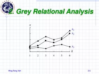
2. Grey Relational Analysis. x. x 1. x 2. x 3. k. 2.1: Grey Relational Analysis. x 0 ={ x 0 (1), x 0 (2),…, x 0 ( n )}: reference sequence x i ={ x i (1), x i (2),…, x i ( n )}: comparative sequence i = 1,2,…, m . Grey relational coefficient : ( x 0 ( k ) , x i ( k ) )

2. Grey Relational Analysis
E N D
Presentation Transcript
2. Grey Relational Analysis x x1 x2 x3 k
2.1: Grey Relational Analysis • x0={x0(1), x0(2),…, x0(n)}: reference sequence • xi={xi(1), xi(2),…, xi(n)}: comparative sequence i = 1,2,…,m. • Grey relational coefficient: (x0(k), xi(k)) (x0(k), xi(k)) = [min+max] [0i(k)+max] 0i(k)=x0(k) xi(k), : distinguish coefficient max=maxi maxkx0(k) xi(k), 0 1, min=mini minkx0(k) xi(k).
Grey Relational Analysis • Grey relational grade: (x0, xi) • 0 (x0(k), xi(k)) 1. • 0 (x0, xi) 1. • Describes the posture relationships between one main factor (reference series) and all other factors (comparison series) in a given system.
Axioms of GRA • Norm Interval (x0(k), xi(k))(0,1], k. (x0(k), xi(k)) = 1, iff x0(k) =xi(k), k. (x0(k), xi(k)) = 1, iff x0,xi . • Duality Symmetric (x0(k), xi(k)) = (xi(k), x0(k)) , iff X = {x0,xi}.
Axioms of GRA • Wholeness (x0(k), xi(k)) (xi(k), x0(k)) almost always, iff X = {xj j = 0,1,…,m, m 2}. • Approachability (x0(k), xi(k)) decreases along with (k) increasing,where (k) = [(x0(k) xi(k))2]1/2 =x0(k) xi(k).
2.2: Grey Generating Space Based on the concept and generating schemes of grey system theory, thedisorderly raw data can • be turned to a regular series for grey modeling. • be transferred to a dimensionless series for grey analyzing. • be changed into a unidirectional series for decision making.
灰關聯因子集 • 假設 X 為序列 xi = {xi(1), xi(2),…, xi(n)}, 其中i = 1,2,…, m, 所構成之集合。 • 若P(X)為一灰關聯因子集,則 xi P(X) 。 • 為使序列具有可以比較之特性,以利灰關聯分析的進行,則序列 xi必須滿足下列三個條件: • 無因次性(Normalization):不論因子xi(k)之測度單位為何,必須經過處理使其成為無因次性(去除單位)。 • 同等級性(Scaling):各序列xi中之xi(k)值均屬同等級或等級相差不大(等級相差不超過2)。 • 同級性(Polarization):序列中的因子描述應為同方向。
Grey Generating Operations An original sequencex= {x(1), x(2),…, x(n)} The generating sequence y= {y(1), y(2),…, y(n)} • Initializing operation: y(k) = x(k) x(1) • Averaging operation: y(k) = x(k) xave, • Maximizing operation: y(k) = x(k) xmax • Minimizing operation: y(k) = x(k) xmin • Intervalizing operation: y(k) = [x(k) xmin] [xmax xmin]
Example 2.1 • x= {4, 2, 6, 8}; xave= 5, xmax= 8, xmin= 2.
Accumulated Generating Operation (AGO) An original sequence x(0)={x(0)(1), x(0)(2),…, x(0)(n)}, x(0)(k) ≧0. • The 1st order AGO (1-AGO): AGO•x(0) = x(1) • The jth order AGO (j-AGO):
Inverse AGO (IAGO) (0)(x(r)(k)) = x(r)(k). (1)(x(r)(k)) = (0)(x(r)(k)) (0)(x(r)(k1)). ( j)(x(r)(k)) = ( j1)(x(r)(k)) ( j1)(x(r)(k1)). • IAGO•x(1) = x(0) = (1)(x(1)) • x(0)(1) = x(1)(1),x(0)(k) = x(1)(k) x(1)(k1) , k=2,3,…,n • Mean generating operation: z(1)(k) =0.5[ x(1)(k) + x(1)(k1)], k=2,3,…,n
x(0)(k) x(1)(k) 7.5 3 4.5 2 3 1 2 1 3 4 k 1 k 1 2 3 4 Example 2.2 • x(0)={x(0)(1), x(0)(2), x(0)(3), x(0)(4)}={1,2,1.5,3} • x(1)={x(1)(1), x(1)(2), x(1)(3), x(1)(4)}={1,3,4.5,7.5}
AGO Effect • The non-negative, smooth, discrete function can be transferred into a series, extended according to an approximate exponential law (grey exponential law). • Thedisorderly raw data can be turned to a regular series for grey modeling.
Weather Analysis Step 1: Data Processing – Initializing 降雨量: x0={1,1.176,1.457,1.151,1.575,1.738,1.135,1.608,2.118,1.425,1.077,0.824} 降雨天數: x1={1,0.938,1,0.813,0.938,0.813,0.500,0.625,0.750,0.750,0.875,0.875} 平均氣溫: x2={1,1.020,1.154,1.423,1.651,1.805,1.940,1.926,1.805,1.597,1.369,1.128} 相對濕度: x3={1,1.024,1.024,1.012,1.012,1.012,0.963,0.963,0.963,0.851,0.963,0.988}
Weather Analysis Step 2: Compute0i(k)=x0(k) xi(k) and then Find maxandmin 01={0,0.238,0.457,0.338,0.638,0.926,0.635,0.983,1.368,0.675,0.202,0.051} 02={0,0.156,0.303,0.272,0.076,0.067,0.805,0.318,0.313,0.173,0.293,0.303} 03={0,0.152,0.433,0.139,0.563,0.726,0.172,0.645,1.155,0.473,0.113,0.164} max=1.368, min=0
Weather Analysis Step 3: Find the Grey Relational Coefficients Let =0.5
Weather Analysis Step 4: Calculate the Grey Relational Grades Average the grey relational coefficients then r(x0,x1)=0.619, r(x0,x2)=0.755, r(x0,x3)=0.687 Step 5: Sort the Grey Relational Grades r(x0,x2) r(x0,x3) r(x0,x1) Note: x0=降雨量, x1=降雨天數,x2=平均氣溫, x3=相對濕度
Example 2.4 Data Pre-processing: x1 = {1.0000, 1.0000, 1.0000, 1.0000} x2 = {1.1759, 0.9375, 1.0201, 1.0244} x3 = {1.4572, 1.0000, 1.1544, 1.0244} x4 = {1.1509, 0.8125, 1.4228, 1.0122}
Weather Analysis 2 Grey Relational Coefficients: = 0.8 r12 = 0.8537, r21 =0.8388 Among four months, January and February are very alike. In general, rij rji
Multi-Reference Sequences Reference sequences: yi={yi(1), yi(2),…, yi(n)} Comparison sequence: xj={xj(1), xj(2),…, xi(n)} i=1,2,…,p; j=1,2,…,q. • Grey relational coefficient: (yi(k), xj(k)) (yi(k), xj(k)) = [min+max] [ij(k)+max] ij(k) =yi(k) xj(k), : distinguish coefficient max=maxi maxj maxk ij(k), 0 1, min=mini minj mink ij(k). • Grey Relational Grade: (yi, xj)
Example 2.5 Data Pre-processing: x1 = {1, 0.889, 0.865, 0.849} y1 x2 = {1, 1.010, 1.017, 1.027} y2 x3 = {1, 0.990, 1.086, 1.042} x4 = {1, 1.529, 1.467, 1.510}
Numerical Example Compute0i(k): 13={0, 0.101, 0.221, 0.193}; 14={0, 0.640, 0.602, 0.661} 23={0, 0.020, 0.067, 0.015}; 24={0, 0.519, 0.450, 0.483} max = 0.661, min = 0. If = 0.5, then • (y2, x3) = 0.932最大,故運輸業x3對工業y2之影響最大。 • ,最強參考列y2 。 • ,最強比較列x3 。