Advanced Computational Techniques for Sequence Alignment in Molecular Biology
160 likes | 286 Vues
This lecture focuses on the optimization of sequence alignment, a fundamental task in computational molecular biology. It delves into dynamic programming approaches, evaluating similarity and distance between nucleotides and residues, and discusses the parsimony alignment method as well as complexity considerations. The material covers homology and non-homology assessments, alignment distances, and heuristics for improving algorithm efficiency. Key algorithms, such as Smith-Waterman and global alignment techniques, will also be explored for their impact on molecular evolution studies.

Advanced Computational Techniques for Sequence Alignment in Molecular Biology
E N D
Presentation Transcript
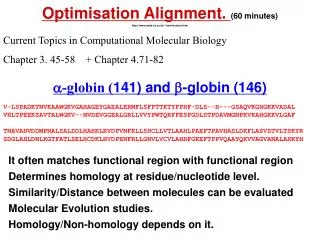
Optimisation Alignment. (60 minutes) http://www.stats.ox.ac.uk/~hein/lectures.htm Current Topics in Computational Molecular Biology Chapter 3. 45-58 + Chapter 4.71-82 a-globin (141) and b-globin (146) V-LSPADKTNVKAAWGKVGAHAGEYGAEALERMFLSFPTTKTYFPHF-DLS--H---GSAQVKGHGKKVADAL VHLTPEEKSAVTALWGKV--NVDEVGGEALGRLLVVYPWTQRFFESFGDLSTPDAVMGNPKVKAHGKKVLGAF TNAVAHVDDMPNALSALSDLHAHKLRVDPVNFKLLSHCLLVTLAAHLPAEFTPAVHASLDKFLASVSTVLTSKYR SDGLAHLDNLKGTFATLSELHCDKLHVDPENFRLLGNVLVCVLAHHFGKEFTPPVQAAYQKVVAGVANALAHKYH It often matches functional region with functional region Determines homology at residue/nucleotide level. Similarity/Distance between molecules can be evaluated Molecular Evolution studies. Homology/Non-homology depends on it.
Number of alignments, T(n,m) 1 9 41 129 321 681 T 1 7 25 63 129 231 G 1 5 13 25 41 61 T 1 3 5 7 9 11 T 1 1 1 1 1 1 C T A G G Alignments columns are equivalent to step (0,1), (1,0) and (1,1) in a [0,n][0,m] matrix. T(n,m) is the number of alignments of s1[1,n] and s2[1,m] then T(n,m)=T(n-1,m)+T(n,m-1)+T(n-1,m-1) T(0,0)=1 T(n,m) > 3 min(n,m) Thus alignment by alignment search for best alignment is not realistic. -n n- n- -n is equivalent to If then alignments are equivalent to choosing two subsets of s1 and and s2 that has to be matched, thus
Parsimony Alignment of two strings. Sequences: s1=CTAGG s2=TTGT. 5, indels (g) 10. Basic operations: transitions 2 (C-T & A-G), transversions 5, indels (g) 10. CTAG CTA G = + TT-G TT- G Cost Additivity {CTA,TT}AL + GG (A) 0 12 Min [ ] {CTA,TTG}AL + G- (B) {CTAG,TTG}AL = 10 4 12 {CTAG,TT}AL + -G (C) 10 32 Di,j=min{Di-1,j-1 + d(s1[i],s2[j]), Di,j-1 + g, Di-1,j +g} Initial condition: D0,0=0. (Di,j := D(s1[1:i], s2[1:j]))
T G T T C T A G G 40 32 22 14 9 17 30 22 12 4 22 20 12 212 22 32 10 2 10 20 30 40 10 20 30 40 50 12 0 CTAGG Alignment: i v Cost 17 TT-GT
Complexity of Accelerations of pairwise algorithm. e { Dynamical Programming: (n+1)(m+1)3=O(nm) Backtracking: O(n+m) Recursion without memory: T(n,m) > 3 min(n,m) Exact acceleration (Ukkonen,Myers). Assume all events cost 1. If de(s1,s2) <2e+|l1-l2|, then d(s1,s2)= de(s1,s2 Heuristic acceleration: Smaller band & larger acceleration, but no guarantee of optimum.
Close-to-Optimum Alignments (Waterman & Byers, 1983) Alignments within of optimal Ex. = 2. 40 32 22 14 9 * 17 T * / 30 22 12 4 12 22 G * / 20 12 2 - 12 22 32 T / 10 2 10 20 30 40 T / 0 10 20 30 40 50 C T A G G C T A G G i i v g Cost 19 T T G T - Caveat: There are enormous numbers of suboptimal alignments.
Hirschberg & Close-to-Optimum Alignments (Hirschberg, 1975). Sets of positions that are on some suboptimal alignment. Alignments within of optimal. Ex. = 2 40/50 32/40 22/30 14/20 9/10 17/0 T 30/40 22/30 12/25 4/15 12/5 22/10 G 20/35 12/25 2/15 12/5 22/10 32/20 T 10/25 2/15 10/15 20/15 30/20 40/30 T 0/17 10/15 20/20 30/25 40/30 50/40 C T A G G Mid point:(3,2) and the alignment problem is then reduced to 2 smaller alignment problems: (CTA + TT) and (GG + GT)
Longer Indels TCATGGTACCGTTAGCGT GCA-----------GCAT gk :cost of indel of length k (for instance 10 + log k) Di,j = min { Di-1,j-1 + d(s1[i],s2[j]), Di,j-1 + g1,Di,j-2 + g2,, Di-1,j + g1,Di-2,j + g2,, } (i-2,j) (i-1,j) (i,j) (i-1,j-1) (i,j-1) Initial condition: D0,0=0 Cubic running time. Quadratic memory. (i,j-2) Comment: Evolutionary Consistency Condition: gi + gj > gi+j
Distance-Similarity (Smith-Waterman-Fitch,1982) Si,j=max{Si-1,j-1 + s(s1[i],s2[j]), Si,j-1 - w, Si-1,j–w} Similarity Distance s(n1,n2) M - d(n1,n2) w 1/(2*M) + g Similarity: Transversions:0 Transitions:3 Identity:5 Indels: 10 + 1/10 Distance: Transitions:2 Transversions 5 Identity 0 Indels:10. M largest dist (5) 40/-40.4 32/-27.3 22/-12.2 14/0.9 9/11.0 17/2.9 T 30/-30.3 22/-17.2 12/-2.1 4/11.0 12/2.9 22/-7.2 G 20/-20.2 12/-7.1 2/8.012/-2.1 22/-12.2 32/-22.3 T 10/-10.1 2/3.0 10/-7.1 20/-17.2 30/-27.3 40/-37.4 T 0/0 10/-10.1 20/-20.2 30/-30.3 40/-40.4 50/-50.5 C T A G G 1. The Switch from Dist to Sim is highly analogous to Maximizing {-f(x)} instead of Minimizing {f(x)}. 2. Dist will based on a metric: i. d(x,x) =0, ii. d(x,y) >=0, iii. d(x,y) = d(y,x) & iv. d(x,z) + d(z,y) >= d(x,y). There are no analogous restrictions on Sim, giving it a larger parameter space.
Local alignment Smith,Waterman (1981 Global Alignment:Si,j=max{Di-1,j-1 + s(s1[i],s2[j]), Si,j-1 -w, Si-1,j-w} Local: Si,j=max{Di-1,j-1 + s(s1[i],s2[j]), Si,j-1 -w, Si-1,j-w,0} 0 1 0 .6 1 2 .6 1.6 1.6 3 2.6 Score Parameters: C 0 0 1 0 1 .3 .6 0.6 2 3 1.6 Match: 1 A 0 0 0 1.3 0 1 1 2 3.3 2 1.6 Mismatch -1/3 G / 0 0 .3 .3 1.3 1 2.3 2.3 2 .6 1.6 Gap 1 + k/3 C / 0 0 .6 1.6 .3 1.3 2.6 2.3 1 .6 1.6 GCC-UCG U / GCCAUUG 0 0 2 .6 .3 1.6 2.6 1.3 1 .6 1 A ! 0 1 .6 0 1 3 1.6 1.3 1 1.3 1.6 C / 0 1 0 0 2 1.3 .3 1 .3 2 .6 C / 0 0 0 1 .3 0 0 .6 1 0 0 G / 0 0 0 .6 1 0 0 0 1 1 2 U 0 0 1 .6 0 0 0 0 0 0 0 A 0 0 1 0 0 0 0 0 0 0 0 A 0 0 0 0 0 0 0 0 0 0 0 C A G C C U C G C U U
Alignment of three sequences. A C ? A s1=ATCG s2=ATGCC s3=CTCC A A C Alignment: AT-CG ATGCC CT-CC Consensus sequence: ATCC Configurations in an alignment column: - - n n n - n - - n - n - n n - n - - - n n n - Recursion:Di,j,k = min{Di-i',j-j',k-k' + d(i,i',j,j',k,k')} Initial condition: D0,0,0 = 0. Running time: l1*l2*l3*(23-1) Memory requirement: l1*l2*l3 New phenomena: ancestral/consensus sequence.
Parsimony Alignment of four sequences C G G C s1=ATCG s2=ATGCC s3=CTCC s4=ACGCG Alignment: AT-CG ATGCC CT-CC ACGCG G C C G Configurations in alignment columns: - - - n - - - n n n - n n n n - - - n - n n - n - - n - n n n - - n - - n - n - n - n n - n n - n - - - - n n - - n n n n - n - Recursion:Di= min{Di-∆ + d(i,∆)} ∆ [{0,1}4\{0}4] Initial condition: D0 = 0.Memory : l1*l2*l3*l4 Computation time: l1*l2*l3*l4*24Memory : l1*l2*l3*l4 New Phenomena: Cost and alignment is phylogeny dependent
Alignment of many sequences. s1=ATCG, s2=ATGCC, ......., sn=ACGCG Alignment: AT-CG ATGCC ..... ..... ACGCG s1 s3 s4 \ ! / ---------- / \ s2 s5 Recursion: Di=min{Di-∆ + d(i,∆)} ∆ [{0,1}n\{0}n] Configurations in an alignment column: 2n-1 Initial condition: D0,0,..0 = 0. Computation time: ln*(2n-1)*n Memory requirement: ln (l:sequence length, n:number of sequences)
Progressive Alignment (Feng-Doolittle 1987 J.Mol.Evol.) Can align alignments and given a tree make a multiple alignment. * * alkmny-trwq acdeqrt akkmdyftrwq acdehrt kkkmemftrwq [ P(n,q) + P(n,h) + P(d,q) + P(d,h) + P(e,q) + P(e,h)]/6 * * *** * * * * * * Sodh atkavcvlkgdgpqvqgsinfeqkesdgpvkvwgsikglte-glhgfhvhqfg----ndtagct sagphfnp lsrk Sodb atkavcvlkgdgpqvqgtinfeak-gdtvkvwgsikglte—-glhgfhvhqfg----ndtagct sagphfnp lsrk Sodl atkavcvlkgdgpqvqgsinfeqkesdgpvkvwgsikglte-glhgfhvhqfg----ndtagct sagphfnp lsrk Sddm atkavcvlkgdgpqvq -infeak-gdtvkvwgsikglte—-glhgfhvhqfg----ndtagct sagphfnp lsrk Sdmz atkavcvlkgdgpqvq— infeqkesdgpvkvwgsikglte—glhgfhvhqfg----ndtagct sagphfnp Lsrk Sods vatkavcvlkgdgpqvq— infeak-gdtvkvwgsikgltepnglhgfhvhqfg----ndtagct sagphfnp lsrk Sdpb datkavcvlkgdgpqvq—-infeqkesdgpv----wgsikgltglhgfhvhqfgscasndtagctvlggssagphfnpehtnk sddm Sodb Sodl Sodh Sdmz sods Sdpb
Summary • Comparison of 2 Strings • Minimize Distance-Maximize Similarity • Dynamical Programming Algorithm • Local alignment • Close-to-Optimal Solutions • Comparison of many Strings • Simultaneous Phylogeny and Alignment