Probe analysis and data preprocessing
Probe analysis and data preprocessing. Affymetrix Probe level analysis Normalization Constant, Loess, Rank invariant, Quantile normalization Expression measure MAS 4.0, LI-Wong ( dChip ), MAS 5.0, RMA Background adjustment PM-MM, PM only, RMA, GC-RMA Statistical analysis of cDNA array

Probe analysis and data preprocessing
E N D
Presentation Transcript
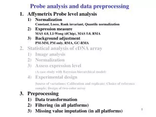
Probe analysis and data preprocessing • Affymetrix Probe level analysis • Normalization • Constant, Loess, Rank invariant, Quantile normalization • Expression measure • MAS 4.0, LI-Wong (dChip), MAS 5.0, RMA • Background adjustment • PM-MM, PM only, RMA, GC-RMA • Statistical analysis of cDNA array • Image analysis • Normalization • Assess expression level • (A case study with Bayesian hierarchical model) • Experimental design • Source of variations; Calibration and replicate; Choice of reference sample; Design of two-color array • Preprocessing • Data transformation • Filtering (in all platforms) • Missing value imputation (in all platforms)
Image analysis Preprocessing (Normalization, filtering, MV imputation) Data visualization Pathway analysis Regulatory network Identify differentially expressed genes Clustering Classification Statistical Issues in Microarray Analysis Experimental design Integrative analysis & meta-analysis
Data Preprocessing • Preliminary analyses extract and summarize information from the microarray experiments. • These steps are irrelevant to biological discovery • But are for preparation of meaningful down-stream analyses for targeted biological purposes. (i.e. DE gene detection, classification, pathway analysis…) • From scanned images • Image analysis (extract intensity values from the images) • Probe analysis (generate data matrix of expression profile) • Preprocessing (data transformation, gene filtering and missing value imputation)
Overview of the technology Hybridization from Affymetrix Inc.
25-mer unique oligo mismatch in the middle nuclieotide Array Design multiple probes (11~16) for each gene from Affymetrix Inc.
Array Probe Level Analysis Background adjustment Normalization Summarization Normalization Background adjustment Summarization • Give an expression measure for each probe set on each array (how to pool information of 16 probes?) • The result will greatly affect subsequent analysis (e.g. clustering and classification). If not modeled properly, => “Garbage in, garbage out” We will leave the discussion of “backgound adjustment” to the last because there’re more new exciting & technical advances.
1.1 Normalization The need for normalization: Intensities of array 2 is intrinsically larger than array 1. (about two fold)
1.1. Normalization • Reason: • Different labeling efficiency. • Different hybridization time or hybridization condition. • Different scanning sensitivity. • ….. Normalization is needed in any microarray platform. (including Affy & cDNA)
1.1. Normalization Constant scaling • Distributions on each array are scaled to have identical mean. • Applied in MAS 4.0 and MAS 5.0 but they perform the scaling after computing expression measure.
1.1. Normalization Constant scaling: Underlying reasoning
1.1 Normalization M-A plot M=0 M A
1.1 Normalization M-A plot shows the need for non-linear normalization. The normalization factor is a function of the expression level.
1.1 Normalization Fit by ‘Lowess’ function in S-Plus Replicate arrays The same pool of sample is applied Normalized Log ratio:
1.1 Normalization Non-linear scaling: Underlying reasoning log relative expression level
1.1 Normalization Non-linear scaling: Underlying reasoning (cont’d) Suppose we know the green genes are non-differentially expressed genes, The problem is: we usually don’t know which genes are constantly expressed!!
1.1. Normalization Loess (Yang et al., 2002) • Using all genes to fit a non-linear normalization curve at the M-A plot scale. (believe that most genes are constantly expressed) • Perform normalization between arrays pairwisely. • Has been extended to perform normalization globally without selecting a baseline array but then is time-consuming.
1.1. Normalization Invariant set (dChip) • Select a baseline array (default is the one with median average intensity). • For each “treatment” array, identify a set of genes that have ranks conserved between the baseline and treatment array. This set of rank-invariant genes are considered non-differentially expressed genes. • Each array is normalized against the baseline array by fitting a non-linear normalization curve of invariant-gene set. Tseng et al., 2001
1.1. Normalization Invariant set (dChip) Advantage: More robust than fitting with all genes as in loess. Especially when expression distribution in the arrays are very different. Disadvantage: The selection of baseline array is important.
1.1. Normalization Quantile normalization (RMA) (Irizarry2003) • Given n array of length p, form X of dimension p×nwhere each array is a col21umn. • 2. Sort each column of X to give Xsort. • 3. Take the means across rows of Xsort and assign this mean to each element in the row to get Xsort. • 4. Get Xnormalized by rearranging each column of Xsort to have the same ordering as original X. X Xsort Xsort Xnormalized
1.1. Normalization Bolstad, B.M., Irizarry RA, Astrand, M, and Speed, TP (2003), A Comparison of Normalization Methods for High Density Oligonucleotide Array Data Based on Bias and Variance Bioinformatics. 19(2):185-193 A careful comparison of different normalization methods and concluded that quantile normalization generally performs the best.
1.2. Summarize Expression Index There’re multiple probes for one gene (11 PM and 11 MM) in U133. How do we summarize the 24 intensity values to a meaningful expression intensity for the target gene?
1.2. Summarize Expression Index • MAS 4.0 • For each probe set, (I: # of arrays, J: # of probes) • PMij-MMij= i+ ij, i=1,…,I, j=1,…,J • iestimated by average difference • Negative expression • Noisy for low expressed genes • Not account for probe affinity
1.2. Summarize Expression Index • dChip (DNA chips) • For each probe set, (I: # of arrays, J: # of probes) • PMij=j + ij + ij + ij • MMij=j + ij + ij • PMij - MMij= ij + ij, i=1,…,I, j=1,…,J • j = J, ij ~ N(0, 2) • Account for probe affinity effect, j. • Outlier detection through multi-chip analysis • Recommended for more than 10 arrays • Multiplicative model: PMij - MMij= ij + ij (better) • Additive model: PMij - MMij= i + j + ij Li and Wong (PNAS, 2001)
1.2. Summarize Expression Index • MAS 5.0 • For each probe set, (I: # of arrays, J: # of probes) • log(PMij-CTij)=log(i)+ij, i=1,…,I, j=1,…,J • CTij=MMij if MMij<PMij • if MMijPMij • i estimated by a robust average (Tukey biweight). • No more negative expression • Taking log adjusts for dependence of variance on the mean. less than PMij
1.2. Summarize Expression Index • RMA (Robust Multi-array Analysis) • For each probe set, (I: # of arrays, J: # of probes) • log(T(PMij))= i + j + ij, i=1,…,I, j=1,…,J • T is the transformation for background correction and normalization • ij ~ N(0, 2) • Log-scale additive model • Suggest not to use MM • Fit the linear model robustly (median polish) Irizarry et al. (NAR, 2003)
R2=0.85 R2=0.95 20g 20g 1.25g 1.25g Affymetrix Latin square data R2=0.97 20g 1.25g from Irizarry et al. (NAR, 2003)
Affymetrix Latin square data from Irizarry et al. (NAR, 2003)
1.3. Background Adjustment • Direct subtraction: PM-MM MAS4.0, dChip, MAS5.0 Assume the following deterministic model: PM=O+N+S (O: optical noise, N: non-specifi binding) MM=O+N => PM-MM=S>0 Is it true?
MM does not measure background noise of PM • Yeast sample hybridized to human chip • If MM measures non-specific binding of PM well, PMMM. • R2 only 0.5. Many MM>PM • 86 HG-U95A human chips, human blood extracts • Two fork phenomenon at high abundance • 1/3 of probes have MM>PM
1.3. Background Adjustment • Reasons MM should not be used: • MM contain non-specific binding information but also include signal information and noise • The non-specific binding mechanism not well-studied. • MM is costly (take up half space of the array) • Ignore MM dChip has an option for PM-only model In general, PM-only is preferred for both dChip or RMA methods.
1.3. Background Adjustment Consider sequence information Naef & Magnasco, 2003 • 95% of (MM>PM) have purine (A, G) in the middle base. • In the current protocol, only pyrimidines (C, T) have biotin-labeled florescence.
1.3. Background Adjustment Fit a simple linear model: • C > G T > A • Boundary effect Naef & Magnasco, 2003
1.3. Background Adjustment Some chemical explanation of the result: See next page
1.3. Background Adjustment Double strand • Remember from the first lecture: • G-C has three hydrogen bonds. (stronger) • A-T has two hydrogen bonds. (weaker) From: Lodish et al. Fig 4-4
1.3. Background Adjustment • GC-RMA O: optical noise, log-normal dist. N: non-specific binding Wu et al., 2004 JASA h: a smooth (almost linear) function. : the sequence information weight computed form the simple linear model.
Criterion to compare diff. methods • Accuracy • In well-controlled experiment with spike-in genes (such as Latin Square data), accuracy of estimated log-fold changes compared to the underlying true log-fold changes are concerned. (only available in data with spike-in genes) • Precision • In data with replicates, the reproducibility (SD) of the same gene in replicates is concerned. (available in data with replicates)
Probe level analysis in Bioconductor (affy package)
A Simple Case Study Latin Square Data 59 HG-U95A arrays 14 spike-in genes in 14 experimental groups M, N, O, P are replicates and Q, R, S, T another replicates http://www.affymetrix.com/analysis/download_center2.affx
A Simple Case Study • Take the following two replicate groups. • Use Bioconducotr to perform a simple evaluation of different probe analysis algorithms. • Note: This is only a simple demonstration. The evaluation result in this presentation is not conclusive.
A Simple Case Study Average log intensities vs SD log intensities. (M, N, O, P) dChip (PM/MM) MAS5.0 dChip (PM only) RMA GC-RMA (PM only) GC-RMA (PM/MM)
A Simple Case Study Average log intensities vs SD log intensities. (Q, R, S, T) dChip (PM/MM) MAS5.0 dChip (PM only) RMA GC-RMA (PM only) GC-RMA (PM/MM)
A Simple Case Study Average pair-wise correlations between replicates Replicate correlation performance: GCRMA(PM-only)>GC-RMA(PM/MM)> RMA> dChip(PM-only)>>dChip(PM/MM)>>MAS5
Outlying genes that do not fit Li-Wong model A Simple Case Study • RMA greatly improves dChip(PM/MM) but dChip(PM-only) model generally seems a little better than RMA. • Average replicate correlations of RMA (0.9978) is a little better than dChip(PM only) (0.9940 & 0.9966) • dChip(PM only) suffers from a number of outlying genes in the model.
Conclusion: • Technological advances have been made to have smaller probe size and better sequence selection algorithms to reduce # of probes in a probe set. This will enable more biologically meaningful genes on a slide and reduce the cost. • Recent analysis advances have been focused on understanding and modelling hybridization mechanisms. This will allow a better use of MM probes or eventually suggest to remove MMs from the array. • The probe analysis is relatively settled in the field. In the second lab session next Friday, we will introduce dChip and RMAexpress for Affymetrix probe analysis.