Microarrays
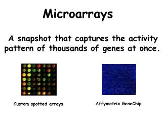
Microarrays. A snapshot that captures the activity pattern of thousands of genes at once. Affymetrix GeneChip. Custom spotted arrays. Practical Applications of Microarrays. Gene Target Discovery By allowing scientists to compare diseased cells with normal cells, arrays can

Microarrays
E N D
Presentation Transcript
Microarrays A snapshot that captures the activity pattern of thousands of genes at once. Affymetrix GeneChip Custom spotted arrays
Practical Applications of Microarrays Gene Target Discovery By allowing scientists to compare diseased cells with normal cells, arrays can be used to discover sets of genes that play key roles in diseases. Genes that are either overexpressed or underexpressed in the diseased cells often present excellent targets for therapeutic drugs. Pharmacology and Toxicology Arrays can provide a highly sensitive indicator of a drug’s activity (pharmacology) and toxicity (toxicology) in cell culture or test animals. This information can then be used to screen or optimize drug candidates prior to launching costly clinical trials. Diagnostics Array technology can be used to diagnose clinical conditions by detecting gene expression patterns associated with disease states in either biopsy samples or peripheral blood cells.
Microarray Platforms • Oligonucleotide-based arrays • 25mers spotted on a glass wafer, Affymetrix GeneChip arrays • Custom spotted 50-80mers generated from • known sequences. • cDNA • Inserts from cDNA libraries • PCR products generated from gene specific or • universal primers
GeneChip® Instrument System Fluidics Station Scanner made by Hewlett-Packard Computer Workstation
* * * * * GeneChip® Probe Arrays Hybridized Probe Cell GeneChip Probe Array Single stranded, fluorescently labeled DNA target 24µm Oligonucleotide probe 1.28cm Each probe cell or feature contains millions of copies of a specific oligonucleotide probe Over 250,000 different probes complementary to genetic information of interest Image of Hybridized Probe Array
Light (deprotection) Mask T T O O O O O O O O HO HO O O O T – Substrate Light (deprotection) Mask C A T A T A G C T G T T C C G T T C C O T T O O O C – Substrate REPEAT Synthesis of Ordered Oligonucleotide Arrays
Probe Tiling StrategyGene Expression (25-mer)
Gene ExpressionTiling Strategy Uninduced Induced 40 separate hybridization events are involved in determining the presence or absence of a transcript 80 separate hybridization events are involved determining differential gene expression of a transcript between two samples
Starting material for Microarrays Platform Affymetrix Poly (A)+ mRNA ~2 mg Total RNA ~10 mg Spotted arrays Poly (A) + ~0.4 – 2 mg Total RNA 10 -100 mg
Agilent Bioanalyzer 2100 Fragmented cRNA Total RNA
B B B B B B B B B B B B Experimental Design Biotin - labeled cRNA transcript Cells Poly (A)+ RNA Or Total RNA IVT Biotin-UTP Biotin-CTP Fragment heat, Mg2+ cDNA Hybridize (16 hours) Wash & Stain Biotin - labeled cRNA fragments Scan (75 minutes) Add Oligo B2 & Staggered Spike Controls (8 minutes)
Normalization and Scaling • Non-biological factors can contribute to the variability of data • in many biological assays, therefore it is important to minimize • the non-biological differences. Factors that may contribute to • variation include: • Amount and quality of target hybridized to array • Amount of stain applied • Experimental variables • The data can be normalized from: • a limited group of probe sets • all probe sets • Thus the normalization of the array is multiplied by a • Normalization Factor (NF) to make its Average Intensity • equivalent to the Average Intensity of the baseline array.
Normalization and Scaling Average intensity of an array is calculated by averaging all the Average Difference values of every probe set on the array, excluding the highest 2% and lowest 2% of the values.
Background Calculation: Measure of non-specific fluorescence attributed to hybridization conditions and sample. Defaults - 16 sectors Horizontal (HZ) : 4 Background • Probe Cells with the lowest 2 % intensity values for each sector are averaged. Vertical (VZ) : 4 Probe Array • This value is subtracted from all cell intensities in each sector before further analysis.
Signal Noise Noise results from small variations in the digitized signal observed by the scanner as it samples the probe array’s surface. The level of the noise is calculated by the software, and then used as one of the criteria to determine the significance of differences between PM and MM probe cells, and differences in probe set intensities across two probe arrays.
Noise Calculation: Q Pixel to pixel variation determined from background Total # of background cells - lowest 2% for each sector. Total # of pixels in a feature i Normalization Factor Standard deviation of the intensities of the pixels making up feature i Scaling Factor Noise for each sector of a given probe array
What determines a positive or negative probe pair? Positive Probe Pair Negative Probe Pair • 1) MM - PM > SDT • and • 2) MM / PM > SRT • 1) PM - MM > SDT • and • 2) PM / MM > SRT PM and MM are similar. No differential signal detected. More MM than PM. Signal is not specific to targeted sequence. PM is more than MM. Yes, this probe pair is detecting a signal.
Statistical Difference Threshold PM - MM > SDT • Calculated by the software based on the noise (Q): SDT = (Q) x (SDTmult) SDTmult (multiplier) is set by default to 2.0 when the single SAPE staining protocol is used (usually with 50 feature arrays), and 4.0 when the antibody amplification protocol is used (usually with 24 feature arrays). (SDTmult) can be modified by user: - increasing makes the analysis more stringent; decreasing less stringent
Statistical Ratio Threshold PM / MM > SRT • SRT is set by user • increasing makes the analysis more stringent; decreasing less stringent • Default SRT value is 1.5 • an SRT threshold value of 1.5 means that the intensity of the PM must be 50% greater than MM (after background subtraction) to meet criteria
Probe Pairs in AverageUsed in calculation of Log Average Ratio and Average Difference Pairs in Average A “Trimmed” probe set prevents outlier probe pairs (extremely positive or negative) from inclusion in calculations for Log Average Ratio (and Average Difference) 8 probe pairs or fewer: Greater than 8 probe pairs: • All probe pairs are used • Super Scoring takes place
Super ScoringUsed in calculation of Log Average Ratio and Average Difference • A mean and a standard deviation are calculated for the intensity differences among an entire probe set. • A filter is then applied to each member of the probe set. • Probe pairs outside of the number of standard deviations set in the parameters are excluded from the calculations of Log Average Ratio and Average Difference • STP is the parameter for setting the number of standard deviations used in Super Scoring. Default Setting is 3 (excludes everything outside of 99.7% of the mean)
Positive Fraction Number of positive probe pairs/total pairs used 15/20 = 0.75
Log Average Ratio Log Avg = 10 * [ log (PM/MM)]/(# Probe Pairs in Average) An average of the log of the intensity ratios is calculated for each probe set from the pairs in average and multiplied by 10.
Positive/Negative Ratio Ratio of positive probe pairs to Negative probe pairs in a probe set Pos/Neg = 18/2 = 9
Average Difference Avg Diff = (PM - MM) / Pairs in Average Average difference is calculated by taking the difference between PM and MM of every probe pair and averaging the differences over the entire probe set. Average difference correlates with expression level Average Difference is not used in the Absolute Call Decision Matrix
Absolute Call Decision Matrix - Absolute Analysis Threshold Values Present 4.0 0.43 1.3 Max Marginal 3.0 0.33 0.9 Min Absent Pos/Neg Ratio Positive Fraction Log Avg Ratio Calls must be in the Present bin in order for quantification metrics to be informative
Increased Probe Pairs & Decreased Probe Pairs Increased Neither Probe Pair Decreased Increased or Probe Pair Decreased
Increased Probe Pair (PM - MM)exp - (PM - MM)base> Change threshold (CT) And [(PM - MM)exp - (PM - MM)base] / (PM - MM)base> (PCT)/100 Probe Set on Baseline Probe Array Probe Set on Experimental Probe Array Increased Probe Pairs Compares changes in relative intensity between two probe pairs on two probe arrays, not positive/negative probe pair changes
Decreased Probe Pair (PM - MM)base - (PM - MM)exp> Change threshold (CT) And [(PM - MM)base - (PM - MM)exp] / (PM - MM)base> (PCT)/100 Probe Set on Baseline Array Probe Set on Experimental Array Decreased Probe Pair Compares changes in relative intensity between two probe pairs on two probe arrays, not positive/negative probe pair changes
Thresholds used in comparison analysis Change Threshold (CT) • The CT can be calculated in either of two ways: • Calculated by the software, based on the SDTs of • the two probe arrays being compared • Calculated as the product of a parameter called • CT multiplier (CTmult) and Q. CTmult is a default setting (80) or can be set by the user • Percent Change Threshold (PCT) • User Defined (default 80); means a probe pair must change 80%
Increase Ratio = # Increased probe pairs / # probe pairs used Decrease Ratio = # Decreased probe pairs / # probe pairs used Increase or Decrease Ratio Probe Set on Baseline Array Probe Set on Experimental Array 10 Increased Probe Pairs / 20 = 0.5 Compares changes in relative intensity between two probe pairs on two probe arrays, not positive/negative probe pair changes
Max (Increase/PP used),(Decrease/PP used) Calculates the number of probe pairs that have changed in a certain direction. Increase/PP used = number of increased probe pairs/number of probe pairs used Decrease/PP used = number of decreased probe pairs/number of probe pairs used Max Inc & Dec = Max (0.95, 0.05) = 0.95 This larger of the values will be used in the decision matrix, which determines whether each transcript’s expression level has changed between baseline and experimental.
Increase/Decrease Ratio Ratio of increase probe pairs over decreased probe pairs Increased: 6 Decreased:1 Inc/Dec = 6/1 = 6
Dpos - Dneg Ratio Dpos-Dneg Ratio= positive change - negative change / # pp used Positive Change = # Positive Probe Pairsexp - # Positive Probe Pairsbase • Dpos - Dneg Ratio flags and excludes probe sets that change in two directions () within one transcript. It also accounts for changes in the neither bin. Negative Change = # Negative Probe Pairsexp - # Negative Probe Pairsbase Probe Set on Baseline Array Probe Set on Experimental Array 7 Positive PP 3 Negative PP 10 Neither 14 Positive PP 4 Negative PP 2 Neither Positive Change = (14 - 7) = 7 Example: Negative Change = (4 - 3) = 1 Dpos -Dneg Ratio = (7 - 1) / 20 = 0.3
Log Average Ratio Change • Log Average is recomputed for each probe set based on probe pairs used in both the baseline and experimental probe arrays. Log Avg Ratio Change = Log Avgexp - Log Avgbase Example: Probe Set on Baseline Array Probe Set on Experimental Array 2probe pairs Not in Average 1probe pair Not in Average Total = 3probe pairs Not in Average Log average is recomputed for each probe set to take into account any probe pairs that have been dropped (not in average) or masked
Differential Call - Comparison Analysis Threshold Values Increase 4.0 0.33 0.2 0.9 Max No Change 3.0 0.43 0.3 1.3 Min Decrease Log Avg Ratio Inc/Dec Ratio Dpos/Total Inc/Total Calls must be in the Increase or Decrease bin in order for quantification metrics to be informative
Average Difference Change • Average Difference is recomputed for each probe set based on common probe pairs to take into account any probe pairs that have been dropped (not in average) or masked Avg Diff Change = Avg Diffexp - Avg Diffbase Average difference change correlates to changes in expression level Average Difference Change is used in Fold Change calculations, but not used in the Comparison Call Decision Matrix
B = A When an “ * ” is present in this column, it signifies that In the baseline array, this transcript was absent. Example: Absolute call B = A Diff Call Define A * I not significant, slight increase from A baseline to A experimental A * D not significant, slight decrease from A baseline to A experimental P * I IMPORTANT, increase in gene expression, A baseline to P exp.
Fold Change:Measure of the relative change in mRNA expression levels between experiments. FC = Avg Diff Change (exp-base) (recomputed) max[ min (Avg Diff exp,Avg Diff base), QM * Qc] + 1 or -1 Lesser of the two values AvgDiffexp AvgDiffbase Defined by the library file AvgDiffexp AvgDiffbase if (QM x QC) of either array is greater than the average difference of the transcript in either the baseline or experimental, the fold change is calculated using the Noise. In this case the fold change is preceded by a (~) and considered an approximation. Greater of the scaled or normalized Qexp or Qbase
Sort Score Based on a calculation that basically multiplies Fold Change and Average Difference Change. The larger the Sort score, the more further away the values are from the noise. Example: Avg. Diff (baseline): 10 Avg. Diff (experimental) :100 Avg. Diff Change : 90 Fold change:10 Avg. Diff (baseline):100 Avg. Diff (experimental): 1000 Avg. Diff Change :900 Fold Change: 10 The fold change in both experiments is 10; however the Sort Score will be approximately 10 times larger in experiment #2 than #1, due to higher average difference change. A fold change with a high sort score means that the average difference change is relatively large.
Save as *.txt file and import into other statistical software programs
Data Visualization: • Data visualization is an important technique for gaining a • fundamental understanding of results of a microarray experiment. • you can detect outliers/anomalies, overall trends, clusters, • correlations with the following visual techniques. • 1-D Profile Plots - e.g. time series response data • Histogram / Frequency Plots - analyze distribution of gene expression data • Star Plots - signature analysis of gene expression profiles • Intensity Plots – color genes by gene expression across all exp’ts at once • Scatter Plots – allow you to visualize high-dimensional microarray data • Integration: • Integrated into your environment by reading files in standard • formats and writing the results out in standard formats. • Import flat files, comma or tab separated Formats, or URL’s • Import from ODBC Data Source • Tiles Saved in Portable Comma Separated (.csv) Format • Automate Via Embedded Tcl Scripting Language • Link to Other Applications by Selecting Data in Spreadsheet or in Graphics.
Data Processing: • Analytical Spreadsheet can Handle Millions of Rows or Columns • Scaling & Normalization (e.g. standardize, log-scale, log & linear scale, power) • Sort rows by Value or by Similarity to Prototype (find genes most similar to • specified prototype) • Missing Data Handling (e.g. analysis, casewise deletion, imputation) • Exploratory Analysis: • New, unexpected discoveries are most easily made during the exploratory • analysis stage. • Cluster analysis – identify genes with similar expression profile • Principal Components Analysis – visually and numerically analyze the correlation • inherent in the data (similarity of genes, of experiments) • Multidimensional Scaling – visually analyze similarity of genes, tissues, or time • points using any one of 20 measures of similarity. • Linear, Non-linear correlation – find significantly correlated genes, tissues, • or time points. • Parametric & Nonparametric tests (e.g. chi-square, t-test, anova, • kolmogorov-smirnov) – genes that are significantly different • Correspondence Analysis – measure the correspondence between (for example) • a cluster analysis grouping and a known functional class of genes. • Randomization Experiments & Permutation Tests – evaluate likelihood of • chance
More Analysis Features • Correlations • Find Genes with expression profiles similar to a chosen Gene • Find Expression Profiles similar to a drawn Profile • Multiple Ways to Define 'Similar' in the 'Find Similar' Search • Quantitative Restrictions • Filter data by degree of expression or x-fold comparisons across experiments. • Find Interesting Genes Function Pathways • Identify Potential New Candidates