Extinction
Extinction. Bruce Walsh jbwalsh@u.arizona.edu Dept. Ecology & Evolutionary Biology University of Arizona. Outline. Death & Destruction: Mass extinctions Extinction: Basic Ecology Theory Genetic Extinction Risks Tools for Assessing extinction risk Management strategies to mitigate risk.

Extinction
E N D
Presentation Transcript
Extinction Bruce Walsh jbwalsh@u.arizona.edu Dept. Ecology & Evolutionary Biology University of Arizona
Outline • Death & Destruction: Mass extinctions • Extinction: Basic Ecology Theory • Genetic Extinction Risks • Tools for Assessing extinction risk • Management strategies to mitigate risk
Greatest Hits: Mass Extinctions Roughly 2 BYA: Most of life on earth wiped out due to pollution (O2) Permian Mass extinction 250 MYA 90 - 95% of marine species became extinct K-T (Cretaceous) Event 65 MYA 85% of all species became extinct End-Ice-Age Mass Extinction (10 TYA) Current on-going mass extinction.
Causes these mass extinctions Massive environmental perturbation Extra-terrestrial impacts Volcanoes Climate change Biological agents
Impact size if S-L 9 had hit Earth (12+ such impacts!) Permian, K-T extinctions Show strong signals of impacts (iridium layer, shock quartz, other signals) Climate change following impact event
Toba extinction event. 75,000 YA Toba, Sumatra, Indonesia
Toba Caldera energy release about one gigaton of TNT 3000 times greater than Mount St. Helens Led to a decrease in average global temperatures by 3 to 3.5 degrees Celsius for several years Believed to have created population bottlenecks in the various homo species that existed at the time Eventually leading to the extinction of all the other homo species except for the branch that became modern humans
Most recent mass extinctions likely human -induced (at least in part) End of ice-age (Quaternary , Holocene) extinctions Extinction of most the the NA/SA mega-fauna Paul Martin’s notion: hunted to extinction by man Others argue for climatic causes Most likely a synergistic interaction between both Many believe we are in “the sixth great mass extinction”
Extinction: Ecological Factors Small population size Declining habitat Changes in other species in the ecosystems What species will save eastern forest wildflowers? Disease
Ecological Theory of Extinction MacArthur-Wilson Theory of Island Biogeography Metapopulation dynamics Demographic Stochasticity
MacArthur-Wilson Island Biogeography (1967) Interested in predicting species numbers on islands Numbers represent a balance between extinction and immigration Prediction: lower extinction rate on larger islands Prediction: higher immigration rates on islands closer to mainland
Size does matter: Species-area curves One of MacArthur & Wilson’s key observation was the species-area curve, predicting the number of species S simply from area A. S = bAz Log(S) = a + z*log(A) Key is species-area exponent z
S (mammals) = 1.188A0.326 S (birds) = 2.526A0.165
Implications of species-area curves S = bAz In theory, one could predict number of species lost given a change in area Suppose area cut in half, equilibrium prediction S* = b(A/2) z S*/S = b(A/2)z / b(A)z = (A/2A)z = (1/2)z Key is species-area exponent z 93% left z = 0.1 87% left z = 0.2 81% left z = 0.3 76% left z = 0.4
This looks somewhat hopefully, as lose some species, but not 50% Flip side of this: Suppose you are designing a reserve and want to convince policy makers to either double or quadruple the current reserve size. How many more species will be added? 2A 4A z 107% 115% 0.1 115% 132% 0.2 123% 151% 0.3 131% 174% 0.4
Complications Species-area slope (z): between islands vs. patches within an island Even if species-area curve exact, only tells us how many species will be lost, NOT which particular ones Nested-set analysis: Look over our “island” to see if species are randomly lost or if some have a greater than average chance of being lost
Non-equilibrium Island Biogeography When isolation is increased, the island is no longer in equilibrium and the number of species is expected to decline Hence, loss of species on ever-isolated islands is expected
Application to conservation biology Isolated patches of habitats are essentially islands Need to maximize patch size Need to maximize exchange between patches When should you NOTmaximize exchange? Risk of disease/pathogens spreading Patches are sufficiently genetically different
Meta-population Analysis Essentially island biogeography with no mainland to serve as a source for immigrants The metapopulation structure assumes the population is distributed as a series of discrete, largely isolated, patches Extinction occurs within a patch, and that patch remains empty until re-colonized by immigrants from other patches At any time, not all patches are occupied. The population persists by being able to colonize patches before all go extinct.
Meta-population Structure Yellow = species present blue = species absent
Sources and Sinks Key features of the metapopulation model Empty patches of habitat are still critical An occupied patch can either be a source or a sink In a source, the long-term growth rate is positive and this patch contributes immigrants to other (potentially empty) patches In a sink, that patch simply absorbs immigrants, and has a net negative growth rate. Cannot tell a source from a sink without long term studies, esp. involving population movement
Counting species numbers Suppose you are trying to estimate the number of species (say moths) in a patch. You have done a number of surveys and have recorded a total of S species S is clearly an underestimate for the actual number T of species that use the patch. How can we estimate this? Simple jackknife estimator: Our estimate of T is just S + number species seen on just one sampling period For example, if we have seen 250 species, 40 of which we only seen in one sampling period, our estimate of T is 250 + 40 = 290.
Departures from the metapopulation model Core-satellite case. A central core source population, with all other patches being sinks. Patchy population case: Even though the population has a patchy distribution, dispersal events are too frequent to allow for extinctions. Here individual patches support parts of a single population (as opposed to the metapopulation structure, where each population is largely separate) Declining population case: Here each subpopulation is a sink, so that the entire population is on its way to extinction.
Key implications from metapopulation model A static snapshot of the population distribution is very misleading Currently unoccupied habitat may be critical for future success An occupied habitat may in fact be a sink, so setting only this area aside as the reserve will doom the species With human intervention, even sink populations are critical, as these can serve as sources to export to currently unoccupied patches
µ ∂ 8 ( ) n 0 d < 1 ° b > d b P = : 0 b < d no = starting size, P = probability of persistence Demographic Stochasticity Random fluctuations of birth and death rates can lead to extinction, even in a population with a positive growth rate Simplest model (but a classic) is due is Ludwig (1971). The net growth rate r is the birth rate (b) minus the death rate (d), r = b - d
Ludwig’s model assumes that the population, if it persists, will growth without limit. Ludwig’s model shows that even a population under positive exponential growth can still go extinct More generally, all populations are finite, and hence all (given enough time) will go extinct As a result, one often tried to estimate the expected time to extinction Such times generally tend to be exponentially distributed Pr(extinction time < t) = 1 - Exp[-t/T(n)] where T(n) is the mean extinction time
Genetic Extinction Risks Inbreeding depression Effective Population size Insufficient Genetic Variation to response Genetic measures of subpopulation isolation
Inbreeding depression Reduction in population fitness due to inbreeding (mating of relatives) Measure of the strength of inbreeding is the inbreeding coefficient, F = Prob(both alleles in an individual are identical by descent) In a finite population, F increases each generation, as F(t+1) = 1/(2N) + [1-1/(2N)]*F(t) Once your population has a non-zero F value, you are stuck with it, EVEN IF THE POPULATION GROWS
Genotypes A1A1 A1A2 A2A2 trait value 0 a+d 2a Freq p2 + Fpq (1-F)2pq q2 + Fpq freq(A1) = p, freq(A2) = q Changes in the mean under inbreeding Increase in homozygotes, decrease in heterozygotes Using the genotypic frequencies under inbreeding, the population mean mF under a level of inbreeding F is related to the mean m0 under random mating by mF = m0 - 2Fpqd
For k loci, the change in mean is Here B is the reduction in mean under complete inbreeding (F=1) , where
Inbred Outbred Inbreeding Depression and Fitness traits
mF m0 - B F m0 0 1 Estimating B In many cases, lines cannot be completely inbred due to either time constraints and/or because in many species lines near complete inbreeding are nonviable In such cases, estimate B from the regression of mF on F, mF = m0 - BF
Observed freq(Heterozygotes) F = 1 - HW freq(Heterozygotes) Estimating F Suppose you have a population under study for listing. How can you estimate the amount of inbreeding it has suffered? Key: Freq(Heterozygotes) = (1-F)2pq
Why do traits associated with fitness show inbreeding depression? • Two competing hypotheses: • Overdominance Hypothesis: Genetic variance for fitness is caused by loci at which heterozygotes are more fit than both homozygotes. Inbreeding decreases the frequency of heterozygotes, increases the frequency of homozygotes, so fitness is reduced. • Dominance Hypothesis: Genetic variance for fitness is caused by rare deleterious alleles that are recessive or partly recessive; such alleles persist in populations because of recurrent mutation. Most copies of deleterious alleles in the base population are in heterozygotes. Inbreeding increases the frequency of homozygotes for deleterious alleles, so fitness is reduced.
Purging Inbreeding Depression If inbreeding depression is caused by deleterious recessives, it may be possible to purge lines of these alleles, provided they are not yet fixed. Strategies have been proposed (expand population and inbred) to attempt to purge captive populations of inbreeding depression, but these remain controversial Natural populations that historically have had small populations may have already purged themselves (to at least some degree) of inbreeding depression. Otherwise they likely would have already gone extinct.
Effective Population size, Ne When the population is not ideal (changes over time, unequal sex ratio, uneven contribution from individuals), we can still compute an effective population size Ne which gives the size of an ideal population that behaves the same as our population We will consider Ne under population bottlenecks unequal sex ratio unequal contribution for all individuals
k N = e k X 1 N ( i ) i =1 Ne under varying population size If the actual population size varies over time, the effective population size is highly skewed towards the smallest value If the populations sizes have been N(1), N(2), …, N(k), the effective population size is given by the harmonic mean Suppose the population sizes are 10000, 10000, 10000, 100. Ne becomes 399
4 N ¢ N * m f N = e N + N m f Ne under unequal sex ratios When there are different number of males (Nm) and females (Nf), the effective population size is skewed towards the rarer sex For example, suppose we used 2 male salmon to fertilize the eggs of 1000 females. What is Ne in this case? Ne = (4*2*1000)/(2 + 1000) = 8