Wavelets and Multiresolution Processing (Wavelet Transforms)
Digital Image Processing. Wavelets and Multiresolution Processing (Wavelet Transforms). Christophoros Nikou cnikou@cs.uoi.gr. Contents. Image pyramids Subband coding The Haar transform Multiresolution analysis Series expansion Scaling functions Wavelet functions Wavelet series

Wavelets and Multiresolution Processing (Wavelet Transforms)
E N D
Presentation Transcript
Digital Image Processing Wavelets and Multiresolution Processing(Wavelet Transforms) Christophoros Nikou cnikou@cs.uoi.gr
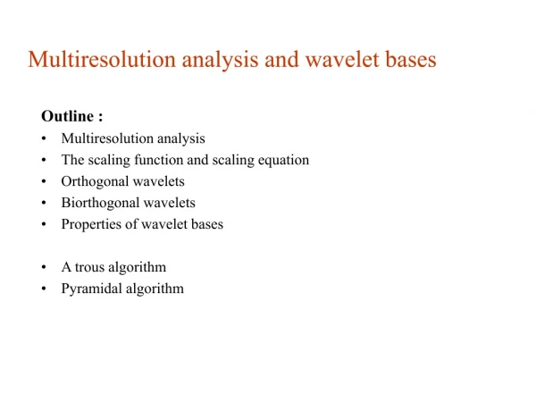
Contents • Image pyramids • Subband coding • The Haar transform • Multiresolution analysis • Series expansion • Scaling functions • Wavelet functions • Wavelet series • Discrete wavelet transform (DWT) • Fast wavelet transform (FWT) • Wavelet packets
1-D Wavelet TransformsThe Wavelet Series A continuous signal may be represented by a scaling function in a subspace and some number of wavelet functions in subspaces Scaling coefficients Detail (wavelet) coefficients
1-D Wavelet TransformsThe Wavelet Series (cont…) Example: using Haar wavelets and starting from j0=0, compute the wavelet series of Scaling coefficients There is only one scaling coefficient for k=0. Integer translations of the scaling function do not overlap with the signal.
1-D Wavelet TransformsThe Wavelet Series (cont…) Example (continued): Detail (wavelet) coefficients
1-D Wavelet TransformsThe Wavelet Series (cont…) Example (continued): Substituting these values:
1-D Wavelet TransformsThe Wavelet Series (cont…) Example (continued): The scaling function approximates the signal by its average value. Each wavelet subspace adds a level of detail in the wavelet series representation of the signal.
1-D Wavelet TransformsThe Discrete Wavelet Transform If the signal is discrete, of length M, we compute its DWT. Scaling coefficients Detail coefficients
1-D Wavelet TransformsThe Discrete Wavelet Transform (cont…) We take M equally spaced samples over the support of the scaling and wavelet functions. Normally, we let j0=0 and M=2J. Therefore, the summations are performed over For Haar wavelets, the discretized scaling and wavelet functions correspond to the rows of the MxMHaar matrix.
1-D Wavelet TransformsThe Discrete Wavelet Transform (cont…) Example: f(n)={1, 4, -3, 0}. We will compute the DWT of the signal using the Haar scaling function and the corresponding wavelet functions. Here, M=4=2J, J=2 and with j0=0 the summations are performed over n=0, 1, 2, 3, j=0, 1 and k=0 for j=0 or k=0, 1 for j=1. The values of the sampled scaling and wavelet functions are the elements of the rows of H4.
1-D Wavelet TransformsThe Discrete Wavelet Transform (cont…) Example (continued): f(n)={1, 4, -3, 0}.
1-D Wavelet TransformsThe Discrete Wavelet Transform (cont…) Example (continued): f(n)={1, 4, -3, 0}. The DWT relative to the Haar scaling and wavelet functions is To reconstruct the signal, we compute for n=0, 1, 2, 3. Notice that we could have started from a different approximation level j00.
1-D Wavelet TransformsThe Fast Wavelet Transform A computationally efficient implementation of the DWT [Mallat 1989]. It resembles subband coding. Consider the multiresolution refinement equation Scaling x by 2j, translating it by k and letting m=2k+n:
1-D Wavelet TransformsThe Fast Wavelet Transform (cont…) The scaling vector hφ may be considered as weights used to expand φ(2jx-k) as a sum of scale j+1 scaling functions. A similar sequence of operations leads to
1-D Wavelet TransformsThe Fast Wavelet Transform (cont…) Injecting these expressions into the DWT formulas yields the following important equations relating the DWT coefficients of adjacent scales.
1-D Wavelet TransformsThe Fast Wavelet Transform (cont…) • Both the scaling and the wavelet coefficients of a certain scale j may be obtained by • convolution of the scaling coefficients of the next scale j+1 (the finer detail scale), with the order-reversed scaling and wavelet vectors hφ(-n)and hψ(-n). • subsampling the result. The complexity is O(M).
1-D Wavelet TransformsThe Fast Wavelet Transform (cont…) The convolutions are evaluated at non-negative even indices. This is equivalent to filtering and downsampling by 2.
1-D Wavelet TransformsThe Fast Wavelet Transform (cont…) The procedure may be iterated to create multistage structures of more scales. The highest scale coefficients are assumed to be the values of the signal itself
1-D Wavelet TransformsThe Fast Wavelet Transform (cont…) The corresponding frequency splitting characteristics for the two-stage procedure.
1-D Wavelet TransformsThe Fast Wavelet Transform (cont…) • Reconstruction may be obtained by the IFWT • upsampling by 2 (inserting zeros). • convolution of the scaling coefficients by hφ(n)and the wavelet coefficients by hψ(n) and summation.
1-D Wavelet TransformsThe Fast Wavelet Transform (cont…) It can also be extended to multiple stages.
1-D Wavelet TransformsRelation to the Fourier Transform • The Fourier basis functions guarantee the existence of the transform for energy signals. • The wavelet transform depends upon the availability of scaling functions for a given wavelet function. • The wavelet transform depends on the orthonormality (biorthogonality) of the scaling and wavelet functions. • The F.T. informs us about the frequency content of a signal. It does not inform us on the specific time instant that a certain frequency occurs. • The W.T. provides information on “when the frequency occurs”.
1-D Wavelet TransformsRelation to the Fourier Transform (cont…) • Heisenberg cells. • The width of each rectangle in (a) represents one time instant. • The height of each rectangle in (b) represents a single frequency. Signal DFT DWT
1-D Wavelet TransformsRelation to the Fourier Transform (cont…) Time domain pinpoints the instance an event occurs but has no frequency information. DFT domain pinpoints the frequencies that are present in the events but provides no time resolution (when a certain frequency appears). Signal DFT DWT
1-D Wavelet TransformsRelation to the Fourier Transform (cont…) In DWT the time-frequency resolution varies but the area of each tile is the same. There is a compromise between time and frequency resolutions. At low frequencies the tiles are shorter (better frequency resolution, less ambiguity regarding frequency) but wider (more ambiguity regarding time). At high frequencies the opposite happens (time resolution is improved). DWT DFT Signal
2-D Discrete Wavelet Transform Extension from 1-D wavelet transforms. A 2-D scaling function and three 2-D wavelet functions are required. They are separable. They are the product of two 1-D functions. Variations along columns Variations along rows Variations along diagonals
2-D Discrete Wavelet Transform (cont…) Given separable scaling and wavelet functions the scaled and translated basis where i is an index and there are two translations m and n.
2-D Discrete Wavelet Transform (cont…) The DWT is given by And the inverse transformation is
2-D Discrete Wavelet Transform (cont…) We take M equally spaced samples over the support of the scaling and wavelet functions. We normally, we let j0=0 and select N=M=2J so that Like the 1-D transform it can be implemented using filtering and downsampling. We take the 1-D FWT of the rows followed by the 1-D FWT of the resulting columns.
2-D Discrete Wavelet Transform (cont…) Reconstruction (inverse 2-D FWT)
2-D Discrete Wavelet Transform (cont…) a) Noisy CT image. We wish to remove the noise by manipulating the DWT. b) Thresholding all of the detail coefficients of the two scale DWT. Significant edge information is eliminated. c) Zeroing the highest resolution detail coefficients (not thresholding the lowest resolution details). d) Information loss in c) with respect to the original image. The edges are slightly disturbed. d) Information loss in e) with respect to the original image. Significant edge information is removed. e) Zeroing all of the detail coefficients of the two scale DWT.
Wavelet Packets • The DWT, as it was defined, decomposes a signal into a sum of scaling and wavelet functions whose bandwidths are logarithmically related. • low frequencies use narrow bandwidths. • high frequencies use wider bandwidths. • For greater flexibility of the partitioning of the time-frequency plane the DWT must be generalized. DWT DFT Signal
Wavelet Packets (cont…) Coefficient tree and subspace analysis tree for the two-scale (three levels) FWT filter bank. The subspace analysis tree provides a more compact representation of the decomposition in terms of subspaces.
Wavelet Packets (cont…) Subspace analysis tree and spectrum splitting for the three-scale (four levels) FWT filter bank. Here, we have three options for the expansion:
Wavelet Packets (cont…) Wavelet packets are conventional wavelet transforms in which the details are filtered iteratively. For example, the three scale wavelet packet tree is Indices A (approximation) and D (detail) denote the path from the parent to the node.
Wavelet Packets (cont…) Filter bank and spectrum (three scale wavelet packet).
Wavelet Packets (cont…) The cost of this generalization increases the computational complexity of the transform from O(M) to O(MlogM). Also, the three scale packet almost triples the number of decompositions available from the three low pass bands.
Wavelet Packets (cont…) The subspace of the signal may be expanded as with spectrum:
Wavelet Packets (cont…) It can also be expanded as with spectrum:
Wavelet Packets (cont…) In general, a P-scale 1-D wavelet packet (associated with P+1 level analysis trees) supports unique decompositions, where D(1)=1 is the initial signal. For instance, D(4)=26 and D(5)=677.
Wavelet Packets (cont…) The problem increases dramatically in 2-D. a P-scale 2-D wavelet packet (associated with P+1 level analysis trees) supports unique decompositions, where D(1)=1 is the initial signal. For instance, D(4)=83.522 possible decompositions. How do we select among them? Impractical to examine each one of them for a given application.
Wavelet Packets (cont…) A common application of wavelets is image compression. Here we will examine a simplified example. We seek to compress the fingerprint image by selecting the “best” three-scale wavelet packet decomposition.
Wavelet Packets (cont…) A criterion for the decomposition is the image energy Algorithm For each node of the analysis tree, from the root to the leaves: Step 1: Compute the energy of the node (EP) and the energy of its offsprings (EA, EH, EV, ED). Step 2: If EA+EH+EV+ED <EP include the offsprings in the analysis tree as they reduce the initial energy. Otherwise, keep only the parent which is a leaf of the tree.
Wavelet Packets (cont…) Many of the 64 initial subbands are eliminated.