Download
1 / 42
430 likes | 1.04k Vues
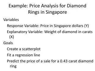
Example: Price Analysis for Diamond Rings in Singapore. Variables Response Variable: Price in Singapore dollars (Y) Explanatory Variable: Weight of diamond in carats (X) Goals Create a scatterplot Fit a regression line Predict the price of a sale for a 0.43 carat diamond ring.

E N D
Example: Price Analysis for Diamond Rings in Singapore Variables Response Variable: Price in Singapore dollars (Y) Explanatory Variable: Weight of diamond in carats (X) Goals Create a scatterplot Fit a regression line Predict the price of a sale for a 0.43 carat diamond ring
diamond.sas (input) odshtmlclose; odshtml; data diamonds; input weight price @@; cards; .17 355 .16 328 .17 350 .18 325 .25 642 .16 342 .15 322 .19 485 .21 483 .15 323 .18 462 .28 823 .16 336 .20 498 .23 595 .29 860 .12 223 .26 663 .25 750 .27 720 .18 468 .16 345 .17 352 .16 332 .17 353 .18 438 .17 318 .18 419 .17 346 .15 315 .17 350 .32 918 .32 919 .15 298 .16 339 .16 338 .23 595 .23 553 .17 345 .33 945 .25 655 .35 1086 .18 443 .25 678 .25 675 .15 287 .26 693 .15 316 .43 . ; data diamonds1; set diamonds; if price ne .;
diamonds.sas (print out) procprintdata=diamonds; run;
diamonds.sas (scatterplot) procsortdata=diamonds1; by weight; symbol1v=circle i=sm70; title1'Diamond Ring Price Study'; title2'Scatter plot of Price vs. Weight with Smoothing Curve'; axis1label=('Weight (Carats)'); axis2label=(angle=90'Price (Singapore $$)'); procgplotdata=diamonds1; plot price*weight / haxis=axis1 vaxis=axis2; run;
diamonds.sas (linear regression line) symbol1v=circle i=rl; title2'Scatter plot of Price vs. Weight with Regression Line'; procgplotdata=diamonds1; plot price*weight / haxis=axis1 vaxis=axis2; run;
diamonds.sas (linear regression) procregdata=diamonds; model price=weight/clbpr; outputout=diagp=predr=resid; id weight; run;
diamonds.sas (linear regression, cont) procprintdata=diag; run;
diamonds.sas (linear regression) procregdata=diamonds; model price=weight/clbpr; outputout=diagp=predr=resid; id weight; run;
diamond.sas (Residual plot) symbol1v=circle i=NONE; title2color=blue 'Residual Plot'; axis2label=(angle=90'Residual'); procgplotdata=diag; plotresid*weight / haxis=axis1 vaxis=axis2 vref=0; where price ne .; run;
Least Squares Solutions b0 = Y̅ - b1X̅
Maximum Likelihood Method Yi ~ N(0 + 1Xi, σ2) L = f1 x f2 x … x fn – likelihood function
Parameter Estimates (SAS) procregdata=diamonds; model price=weight/clb;
Summary of Inference Yi = 0 + 1Xi + I I ~ N(0,σ2) are independent, random errors Parameter Estimators: 0: b0 = Y̅ - b1X̅
Summary of Inference (cont) Reject H0 if the p-value is small (≤ (0.05))
Power: Example (nknw055.sas) Toluca Company (details of study: section 1.6), Response variable: Work hours Explanatory variable: Lot size Assume: 2 = 2500 n = 25 SSXX = 19800 Calculate power when 1 = 1.5
Power: Example (SAS) data a1; n=25; sig2=2500; ssx=19800; alpha=.05; sig2b1=sig2/ssx; df=n-2; beta1=1.5; delta=abs(beta1)/sqrt(sig2b1); tstar=tinv(1-alpha/2,df); power=1-probt(tstar,df,delta)+probt(-tstar,df,delta); output; procprintdata=a1;run;
Power: Example (SAS, cont) data a2; n=25; sig2=2500; ssx=19800; alpha=.05; sig2b1=sig2/ssx; df=n-2; do beta1=-2.0to2.0by.05; delta=abs(beta1)/sqrt(sig2b1); tstar=tinv(1-alpha/2,df); power=1-probt(tstar,df,delta) +probt(-tstar,df,delta); output; end; procprintdata=a2;run; title1'Power for the slope in simple linear regression'; symbol1v=nonei=join; procgplotdata=a2; plot power*beta1; run;
Estimation of E{Yh}: (nknw060.sas) data a1; infile'I:\My Documents\Stat 512\CH01TA01.DAT'; input size hours; run; data a2; size=65; output; size=100; output; data a3; set a1 a2; procprintdata=a3; run; procregdata=a3; model hours=size/clm; id size; run; quit;
Estimation of E{Yh(new)}: (nknw065.sas) data a1; infile'H:/Stat512/Datasets/CH01TA01.DAT'; input size hours; data a2; size=65; output; size=100; output; data a3; set a1 a2; procregdata=a3; model hours=size/cli; id size; run;
Confidence Band (nknw065x.sas) dataa1; infile'H:/My Documents/Stat 512/CH01TA01.DAT'; input size hours; data a2; size=65; output; size=100; output; data a3; set a1 a2; procregdata=a3 alpha=0.10; modelhours=size; run; quit;
Confidence Band (nknw067.sas): Example (find t) data a1; n=25; alpha=.10; dfn=2; dfd=n-2; w2=2*finv(1-alpha,dfn,dfd); w=sqrt(w2); alphat=2*(1-probt(w,dfd)); tstar=tinv(1-alphat/2, dfd); CL = 1 - alphat; output; procprintdata=a1;run;
Confidence Band: Example (cont) data a2; infile‘H:/STAT 512/CH01TA01.DAT'; input size hours; title1'90% Confidence Band'; symbol1v=circle i=rlclm97; procgplotdata=a2; plot hours*size; run;
CI vs. Prediction: (still nknw067.sas) *rlclm is for the mean or confidence band (blue) and rlcli is for the individual plots or prediction band (red); title1'90% Confidence Band and prediction band'; title2'Confidence band is in blue and prediction band is in red'; symbol1v=circle i=rlclm97 c=blue; symbol2v=nonei=rlcli97 ci=red; procgplotdata=a1; plot hours*size hours*size/overlay; run; /*The above code is equivalent to proc gplot data=a1; plot hours*size; plot2 hours*size; run; */
ANOVA table: nknw065.sas (modified) data a1; infile'H:/My Documents/Stat 512/CH01TA01.DAT'; input size hours; procregdata=a1; model hours=size; run;
Regression and Causality http://stats.stackexchange.com/questions/10687/does-simple-linear-regression-imply-causation