Understanding Genetic Information and Population Dynamics through Markov Chains
This document provides an overview of genetic concepts including genes, genomes, and chromosomes. It delves into the relationship between genotype and phenotype, exploring how inherited characteristics manifest in individuals. The Fisher-Wright model is introduced to illustrate genetic drift and allele frequency changes over time in a population. Additionally, exercises are proposed to simulate these concepts through programming, allowing for practical engagement with the mechanisms of inheritance and population genetics.

Understanding Genetic Information and Population Dynamics through Markov Chains
E N D
Presentation Transcript
Genetic Information • Gene – basic unit of genetic information. Genes determine the inherited characters. • Genome – the collection of genetic information. • Chromosomes – storage units of genes. • DNA - is a nucleic acid that contains the genetic instructions specifying the biological development of all cellular forms of life
Locus1 Possible Alleles: A1,A2 Locus2 Possible Alleles: B1,B2,B3 Chromosome Logical Structure • Locus – location of a gene/marker on the chromosome. • Allele – one variant form of a gene/marker at a particular locus.
Human Genome Most human cells contain 46 chromosomes: • 2 sex chromosomes (X,Y): XY – in males. XX – in females. • 22 pairs of chromosomes named autosomes.
Genotypes Phenotypes • At each locus (except for sex chromosomes) there are 2 genes. These constitute the individual’s genotype at the locus. • The expression of a genotype is termed a phenotype. For example, hair color, weight, or the presence or absence of a disease.
GenotypesPhenotypes(example) • Eb- dominant allele. • Ew- recessive allele. genotypes phenotypes
Population genetics • genetic structure of a population • alleles • genotypes group of individuals of the same species that can interbreed Patterns of genetic variation in populations Changes in genetic structure through time
Describing genetic structure • genotype frequencies • allele frequencies rr = white Rr = pink RR = red An example of incomplete dominance
Describing genetic structure • genotype frequencies • allele frequencies genotype frequencies: 200 white 500 pink 300 red 200/1000 = 0.2 rr 500/1000 = 0.5 Rr 300/1000 = 0.3 RR total = 1000 flowers
Describing genetic structure • genotype frequencies • allele frequencies 200 rr 500 Rr 300 RR = 400 r = 500 r =500 R = 600 R allele frequencies: 900/2000 = 0.45 r 1100/2000 = 0.55 R total = 2000 alleles
Fisher-Wright model • Genetic drift: the stochastic fluctuations in allele frequency due to random sampling in a finite population. • The Fisher-Wright model describes the process of genetic drift in a finite population. The model assumes: 1. M diploid organisms (N=2M alleles) 2. Monoecious reproduction (e.g. plants) 3. Non-overlapping generations 4. Random mating 5. No mutation 6. No selection • Given two alleles in a population, a and A, genetic drift describes their change in frequency over time.
Fisher-Wright model This model assumes a fixed population of size N=2M genes composed of a and Aalleles (at one locus). The makeup of the next generation is determined by N independent binomial samples as follows: if the parent population consists of j alleles of type a and N −j alleles of type A, then each sample results in a or A with probabilities: respectively. Repeated selections are done with replacement. We thus generate a Markov chain where Xt is the number of a-genes in the tth generation. The state space contains the N+1 values {0, 1, 2, ...,N}.
Exercise • Write a program to simulate the Fisher-Wright model in which the population is represented explicitlyas a vector of ones(a) and zeros(A). • Proceed by writing a function: function r = single_sim(N,j0,nGen) Where N=population size, j0=number of a-alleles in 1st generation, nGen=# of generations The output should look as follows:
Exercise (continued) • Using the function single_sim, write a program to simulate the system 50 times, and estimate the probability that the a- allele reaches fixation (frequency = 1.0) after 35 generations with N=6 for j0=2,4 and 5. • Plot the first six simulations (you can use plot(Y) where Y is matrix). The result should look like this:
Fisher-Wright model • The transition probability matrix for the system is: • Note that states 0 and N are absorbing in the sense that once Xt = 0 or N then no further state change is possible. We are interested in calculating the probability for a particular X0 that a or A will reach fixation, i.e. we will reach a population composed only of a- or A- alleles.
Exercise • Write a function P = buildFWP(N) that constructs the Fisher-Wright transition probability matrix for arbitrary N. Take advantage of the function binomialPMF you have already written. Compute the corresponding matrix for N=6. • Use the eigenvectors method to find the stationary distribution(s). Do they make sense? • Raise P to a large power (e.g. 100). What does this tell us?