Measurements
370 likes | 555 Vues
Measurements. Part 1: Basic Principle of Measurements. Learning objectives. To state sub-systems in a measurement system To understand main function in each sub-system To understand the basic properties of measurement systems. Basic components in a measurement system.

Measurements
E N D
Presentation Transcript
Measurements Part 1: Basic Principle of Measurements
Learning objectives • To state sub-systems in a measurement system • To understand main function in each sub-system • To understand the basic properties of measurement systems
Basic components in a measurement system Basic components in a measurement system are shown below: Amplification and Conditioning It is also important to mention that a power supply is an important element for the entire system.
INSTRUMENTATION CHARACTERISTICS • Shows the performance of instruments to be used. • Divided into two categories: static and dynamic characteristics. • Static characteristics refer to the comparison between steady output and ideal output when the input is constant. • Dynamic characteristics refer to the comparison between instrument output and ideal output when the input changes.
STATIC CHARACTERISTICS • ACCURACY • Accuracy is the ability of an instrument to show the exact reading. • Always related to the extent of the wrong reading/non accuracy. • Normally shown in percentage of error which of the full scale reading percentage.
STATIC CHARACTERISTICS Example : A pressure gauge with a range between 0-1 bar with an accuracy of ± 5% fs (full-scale) has a maximum error of: 5 x 1 bar = ± 0.05 bar 100 Notes: It is essential to choose an equipment which has a suitable operating range.
STATIC CHARACTERISTICS Example : A pressure gauge with a range between 0 - 10 bar is found to have an error of ± 0.15 bar when calibrated by the manufacturer. Calculate : a. The error percentage of the gauge. b. The error percentage when the reading obtained is 2.0 bar.
STATIC CHARACTERISTICS Answer : a. Error Percentage = ± 0.15 bar x 100 = ± 1.5% 10.0 bar b. Error Percentage = ± 0.15 bar x 100 = ± 7.5 % 2.0 bar • The gauge is not suitable for use for low range reading. • Alternative : use gauge with a suitable range.
STATIC CHARACTERISTICS Example : Two pressure gauges (pressure gauge A and B) have a full scale accuracy of ± 5%. Sensor A has a range of 0-1 bar and Sensor B 0-10 bar. Which gauge is more suitable to be used if the reading is 0.9 bar? Answer : Sensor A : Equipment max error = ± 5 x 1 bar = ± 0.05 bar 100 Equipment accuracy @ 0.9 bar ( in %) = ± 0.05 bar x 100 = ± 5.6% 0.9 bar
STATIC CHARACTERISTICS Sensor B : Equipment max error = ± 5 x 10 bar = ± 0.5 bar 100 Equipment accuracy @ 0.9 bar ( in %) = ± 0.5 bar x 100 = ± 55% 0.9 bar Conclusion : Sensor A is more suitable to use at a reading of 0.9 bar because the error percentage (± 5.6%) is smaller compared to the percentage error of Sensor B (± 55%).
2. PRECISION STATIC CHARACTERISTICS • An equipment which is precise is not necessarily accurate. • Defined as the capability of an instrument to show the same reading when used each time (reproducibility of the instrument).
STATIC CHARACTERISTICS Example : X : result Centre circle : true value XXX XXX Low accuracy, high precision XXX XXXX XXX X X X High accuracy, high precision x x Low accuracy, low precision
Accuracy vs Precision High Precision, but low accuracy. There is a systematic error.
Accuracy vs Precision (Cont) High accuracy means that the mean is close to the true value, while high precision means that the standard deviation σ is small.
3. TOLERANCE STATIC CHARACTERISTICS • Closely related to accuracy of an equipment where the accuracy of an equipment is sometimes referred to in the form of tolerance limit. • Defined as the maximum error expected in an instrument. • Explains the maximum deviation of an output component at a certain value.
4. RANGE OF SPAN STATIC CHARACTERISTICS • Defined as the range of reading between minimum value and maximum value for the measurement of an instrument. • Has a positive value e.g..: The range of span of an instrument which has a reading range of –100°C to 100 °C is 200 °C.
5. BIAS STATIC CHARACTERISTICS • Constant error which occurs during the measurement of an instrument. • This error is usually rectified through calibration. Example : A weighing scale always gives a bias reading. This equipment always gives a reading of 1 kg even without any load applied. Therefore, if A with a weight of 70 kg weighs himself, the given reading would be 71 kg. This would indicate that there is a constant bias of 1 kg to be corrected.
6. LINEARITY STATIC CHARACTERISTICS • Maximum deviation from linear relation between input and output. • The output of an instrument has to be linearly proportionate to the measured quantity. • Normally shown in the form of full scale percentage (% fs). • The graph shows the output reading of an instrument when a few input readings are entered. • Linearity = maximum deviation from the reading of x and the straight line.
Linearity Output Readings Measured Quantity
7. SENSIVITY STATIC CHARACTERISTICS • Defined as the ratio of change in output towards the change in input at a steady state condition. • Sensitivity (K) = Δθο Δθi Δθο : change in output; Δθi : change in input Example 1: The resistance value of a Platinum Resistance Thermometer changes when the temperature increases. Therefore, the unit of sensitivity for this equipment is Ohm/°C.
Sensitivity Most sensitive Variation of the physical variables
STATIC CHARACTERISTICS Example 2: Pressure sensor A with a value of 2 bar caused a deviation of 10 degrees. Therefore, the sensitivity of the equipment is 5 degrees/bar. • Sensitivity of the whole system is (k) = k1 x k2 x k3 x .. x kn θo θi k1 k2 k3
STATIC CHARACTERISTICS Example: Consider a measuring system consisting of a transducer, amplifier and a recorder, with sensitivity for each equipment given below: Transducer sensitivity 0.2 mV/°C Amplifier gain 2.0 V/mV Recorder sensitivity 5.0 mV/V Therefore, Sensitivity of the whole system: (k) = k1 x k2 x k3 k = 0.2 mV x 2.0 V x 5.0 mV °C mV V k = 2.0 mV/°C
Example : The output of a platinum resistance thermometer (RTD) is as follows: Calculate the sensitivity of the equipment. Answer : Draw an input versus output graph. From that graph, the sensitivity is the slope of the graph. K = Δθο graph = (400-200) ohm = 2 ohm/°C Δθi slope (200-100) °C
8. DEAD SPACE / DEAD BAND STATIC CHARACTERISTICS • Defined as the range of input reading when there is no change in output (unresponsive system). Output Reading - + Measured Variables Dead Space
9. RESOLUTION STATIC CHARACTERISTICS • The smallest change in input reading that can be traced accurately. • Given in the form ‘% of full scale (% fs)’. • Available in digital instrumentation.
10. THRESHOLD STATIC CHARACTERISTICS • When the reading of an input is increased from zero, the input reading will reach a certain value before change occurs in the output. • The minimum limit of the input reading is ‘threshold’.
DYNAMIC CHARACTERISTICS • Explains the behaviour system of instruments system when the input signal is changed. • Depends on a few standard input signals such as ‘step input’, ‘ramp input’ dan ‘sine-wave input’.
DYNAMIC CHARACTERISTICS Step Input • Sudden change in input signal from steady state. • The output signal for this kind of input is known as ‘transient response’. Input Time
DYNAMIC CHARACTERISTICS Ramp Input • The signal changes linearly. • The output signal for ramp input is ‘ramp response’. Input Time
DYNAMIC CHARACTERISTICS Sine-wave Input • The signal is harmonic. • The output signal is ‘frequency response’. Input Time
Response time One would like to have a measurement system with fast response. In other words, the effect of the measurement system on the measurement should be as small as possible.
EXAMPLE OF DYNAMIC CHARACTERISTICS Response from a 2nd order instrument: Output 100% 90% 10% tr Time
EXAMPLE OF DYNAMIC CHARACTERISTICS Response from a 2nd order instrument: • Rise Time ( tr ) • Time taken for the output to rise from 10% to 90 % of the steady state value. • Settling time (ts) • Time taken for output to reach a steady state value.
Sensor Performance Characteristics • Transfer Function: • The functional relationship between physical input signal and electrical output signal. Usually, this relationship is represented as a graph showing the relationship between the input and output signal, and the details of this relationship may constitute a complete description of the sensor characteristics. For expensive sensors which are individually calibrated, this might take the form of the certified calibration curve. • Sensitivity: • The sensitivity is defined in terms of the relationship between input physical signal and output electrical signal. The sensitivity is generally the ratio between a small change in electrical signal to a small change in physical signal. As such, it may be expressed as the derivative of the transfer function with respect to physical signal. Typical units : Volts/Kelvin. A Thermometer would have "high sensitivity" if a small temperature change resulted in a large voltage change. • Span or Dynamic Range: • The range of input physical signals which may be converted to electrical signals by the sensor. Signals outside of this range are expected to cause unacceptably large inaccuracy. This span or dynamic range is usually specified by the sensor supplier as the range over which other performance characteristics described in the data sheets are expected to apply.
Sensor Performance Characteristics • Accuracy: • Generally defined as the largest expected error between actual and ideal output signals. Typical Units : Kelvin. Sometimes this is quoted as a fraction of the full scale output. For example, a thermometer might be guaranteed accurate to within 5% of FSO (Full Scale Output) • Hysteresis: • Some sensors do not return to the same output value when the input stimulus is cycled up or down. The width of the expected error in terms of the measured quantity is defined as the hysteresis. Typical units : Kelvin or % of FSO • Nonlinearity (often called Linearity): • The maximum deviation from a linear transfer function over the specified dynamic range. There are several measures of this error. The most common compares the actual transfer function with the `best straight line', which lies midway between the two parallel lines which encompasses the entire transfer function over the specified dynamic range of the device. This choice of comparison method is popular because it makes most sensors look the best.
Sensor Performance Characteristics • Noise: • All sensors produce some output noise in addition to the output signal. The noise of the sensor limits the performance of the system based on the sensor. Noise is generally distributed across the frequency spectrum. Many common noise sources produce a white noise distribution, which is to say that the spectral noise density is the same at all frequencies. Since there is an inverse relationship between the bandwidth and measurement time, it can be said that the noise decreases with the square root of the measurement time. • Resolution: • The resolution of a sensor is defined as the minimum detectable signal fluctuation. Since fluctuations are temporal phenomena, there is some relationship between the timescale for the fluctuation and the minimum detectable amplitude. Therefore, the definition of resolution must include some information about the nature of the measurement being carried out. • Bandwidth: • All sensors have finite response times to an instantaneous change in physical signal. In addition, many sensors have decay times, which would represent the time after a step change in physical signal for the sensor output to decay to its original value. The reciprocal of these times correspond to the upper and lower cutoff frequencies, respectively. The bandwidth of a sensor is the frequency range between these two frequencies.