Download
1 / 82
820 likes | 965 Vues
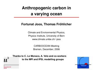
Fortunat Joos, Thomas Fr öhlicher Climate and Environmental Physics, Physics Institute, University of Bern www.climate.unibe.ch /~joos CARBOOCEAN Meeting Bremen, December, 2006 Thanks to C. Lo Monaco, A. Velo and co-workers to the MPI and IPSL modelling groups. Anthropogenic carbon in

E N D
Fortunat Joos, Thomas Fröhlicher Climate and Environmental Physics, Physics Institute, University of Bern www.climate.unibe.ch/~joos CARBOOCEAN Meeting Bremen, December, 2006 Thanks to C. Lo Monaco, A. Velo and co-workers to the MPI and IPSL modelling groups Anthropogenic carbon in a varying ocean
Data from the past show that anthropogenic climate change is proceeding at high speed
The atmospheric concentration of carbon dioxide in 2005 exceeds by far the natural range over the last 650,000 years (180 to 300 ppm) as determined from ice cores (IPCC, SPM, 2007). CO2 versus Antarctic Temperature Natural Range 10000 20000 0 Time (years before present) (IPCC, 2007, Fig. TS-2a)
The age distribution of air enclosed in ice Greenland CH4 Antarctic (Dome C), today Antarctic (Dome C), Last Glacial Maximum (Joos and Spahni, PNAS, submitted)
Rates of Change over the past 22,000 years The rate of increase in the combined radiative forcing from CO2, CH4 and N2O during the industrial era is very likely to have been unprecedented in more than 10,000 years (IPCC, SPM, 2007) (Joos and Spahni, PNAS, submitted)
Models and system understanding: current carbon emissions will affect the climate for many millennia
Long-term CO2 and sea level committment in EMICs 2000 GtC Cumulative Emissions 1820 -2100 60% Atmosphere IPCC AR4 EMIC Intercomparison Plattner et al., J.Clim., 2007; 0% 60% Thermal Expansion (m) Ocean 1 60% Land 0 2000 2500 3000 2000 2500 3000 Year
IPCC Scenario Meeting, Sep 2007 • A new set of emission mitigation and • baseline scenarios • Four scenarios to be selected • for AOGCM runs • → use in CARBOOCEAN
Projected CO2 in 2100 Baseline Mitigation 650 to 950 ppm380 to 620 ppm (Van Vuren et al., submitted)
Projected Radiative Forcing in 2100 Baseline Mitigation Radiative Forcing (W m-2): 6 to 10 2.4 to 5.1 CO2 (ppm): 650 to 950 380 to 620 (Van Vuren et al., submitted)
Projected Temperature Change (1990 to 2100) Baseline Mitigation 2.6 to 4.6°C 1.1 to 2.4°C (Van Vuren et al., submitted)
Ocean Acidification and Aragonite Saturation 4 . 3 supersaturation Observation- based 2 1 WA 0 4 NCAR CSM1.4 3 WA 2 1 0 (Steinacher, 2007)
Evolution of Aragonite Saturation in the Surface 90oN 4 3 supersaturation Latitude 2 1 WA 90oS 0 300 500 700 Surface pCO2 (ppm) (Steinacher, 2007)
Calcite Aragonite Total CaCO3 CaCO3 flux in PISCES (PgC/m2/y) Fluxes of calcite and aragonite to depth 0 Calcite Aragonite Total CaCO3 Depth (m) Will dissolution of shallow aragonite sediments mitigate some of the ocean acidification signal? Magnitude? Time scales? 5000 0.4 0 0.8 CaCO3 Flux (PgC/yr) Gangsto, in prep.
Conclusions: Ocean Acidification 460 ppm: Arctic Ocean becomes undersaturated with respect to Aragonite 560 ppm: Antarctic surface waters become undersaturated 560 ppm: surface water that is more than 3 times oversaturated dissappears
How well do different reconstruction methods of Canth work in the AOGCM model world?
a) Canth simulated by model • b) Canth reconstructed from simulated tracers • (C, Alk, O2, ...) Simulated and reconstructed Canth should be identical
Surface Temperature and CO2 for SRES A2 and B1 2 A2 1 NCAR CSM1.4 Instrumental DT (oC) B1 . 0 • Anthropogenic forcing • - Fossil and land use CO2 emissions • - CH4, N2O, CFCs • direct sulphate aerosols • Natural forcing • solar irradiance • stratospheric volcanic • aerosols 1900 2000 2100 Year 700 A2 CO2 (ppm) 500 Data B1 300 1900 2000 2100 Year
Anthropogenic CO2 Observation-based (GLODAP) NCAR CSM1.4 . 100 50 Canth (mol m-2) 0
Change in decadal-mean PO4 from 1820 to 2000 AD, Atlantic, 20 W 0 40 • No century-scale trends • decadal variabilityin high latitudes of NA Depth (m) 0 DPO4*117 (mmol-C/kg) 4500 -40 80oS 60oN
Modelled evolution of DIC and Canth for an individual grid cell (60 N, 20 W) Remove natural variability in DIC by splining to get Canth 2180 DIC (mmol/m3) Canth DIC 2100 1850 1900 2000 1950 Time
Canth in the Atlantic along 20 W NCAR CSM1.4, 1994 0 70 Depth (m) 30 Canth (mmol-C/kg) 0 -10 5000 80oS 60oN
b) Canth reconstructed from simulated tracers • (Carbon, Alk, O2, ...)
The TrOCA method as an example Total Carbon „Organic Matter Remineralization“ „CaCO3 dissolution“ „preindustrial Total Carbon“ • The usual assumptions • Fixed Redfield ratios to correct for remineralisation • No century-scale trends • time-invariant air-sea disequilibrium
Canth in the Atlantic along 20 W TrOCA with NCAR output, 1994 0 70 Depth (m) 30 Canth (mmol-C/kg) 0 5000 -10 80oS 60oN
a) Canth simulated by model • b) Canth reconstructed from simulated tracers • (T, S, O2, ...) Are simulated and reconstructed Canth identical?
70 (mmol-C/kg) TrOCA-NCAR 0 -10 „truth“, NCAR-Model
Remineralisation and Canth is overestimated in reconstruction TrOCA Remineralisation of organic matter does not consume O2 in oxygen minimum zones (OCMIP Protocoll) Oxygen in NCAR
Anoxic remineralisation of organic matter may bias Canth estimates
70 (mmol-C/kg) TrOCA-MPI 0 -10 „truth“, MPI Model
Negative Canth in deep ocean TrOCA-MPI Century-scale Trend in PO4 in MPI Model
Internal Variability in AOU 5 4 3 sdv of decal averaged AOU (mmol/kg) 2 1 0 Frölicher et al., in prep.
The impact of volcanic forcing on global mean AOU and O2 -DAOU DO2 100 Depth (m) Optical Depth 1500 1960 2000 1960 2000 Year Frölicher et al., in prep.
The impact of volcanic forcing on global meanO2 and AOU -DAOU DO2 100 Depth (m) 1500 1960 2000 1960 2000 Year Frölicher et al., in prep.
Internal Variability in DIC and in DC* from a control run in top 2000 m 1s, DC* 1s, DIC . 4 15 depth (mmol-C/kg) 0 0 -4 -15 60oS 80oN 60oS 80oN Levine et al., in press
Difference between modeled and reconstructed Canth for the DC* method Modelled increase over 10 year Difference (model-reconstruction) . 15 0 -15 60oS 80oN (mmol-C/kg) Levine et al., in press
Both externally-forced and internal variability may bias Canth estimates
Other potential problems? • Parameters of reconstruction method have not • been determined with model output • Fixed Redfield ratios assumed in model – correct?
How do results from different methods compare with modeled Canth?
Reconstruction methods: • TrOCA (Touratier et al.) • CT0 (Vazquez-Rodriguez; • adjusted C* method) • CT0IPSL: (Lo Monaco; back-calculation method, • uses different preformed relationships • for southern and northern water)
TrOCA CT0 70 (mmol-C/kg) IPSL „Truth“: NCAR Model 0 -10
Difference between simulated and reconstructed Canth, 20 W,1994 0 50 TrOCA Depth (m) 0 (mmol-C/kg) -50 5000 80oS 60oN
Difference between simulated and reconstructed Canth, 20 W,1994 0 50 CT0 Depth (m) 0 (mmol-C/kg) -50 5000 80oS 60oN
Difference between simulated and reconstructed Canth, 20 W,1994 0 50 IPSL Depth (m) 0 (mmol-C/kg) -50 5000 80oS 60oN