Download
1 / 48
620 likes | 1.01k Vues
“GIS-integrated Decision Support System (DSS) in Water Resources Management”. Ivan Maximov, Ph.D The Ministry of Natural Resources Russian Federal Water Resources Agency. STRUCTURE OF PRESENTATION 1. DSS (Decision Support Systems)

E N D
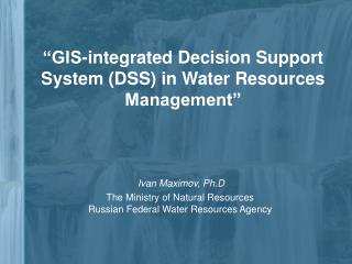
“GIS-integrated Decision Support System (DSS) in Water Resources Management” Ivan Maximov, Ph.D The Ministry of Natural Resources Russian Federal Water Resources Agency
STRUCTURE OF PRESENTATION 1. DSS (Decision Support Systems) 2. U.S EPA BASINS (Better Assessment Science Integrating point and Non-point Sources): Integrated GIS, data analysis and modeling system designed to support watershed based analysis. 3. Application of BASINS. Examples. 4. CONCLUSION
DSS (Decision Support Systems) • Q: What is a Decision Support System? Process? Tool? As a process: …is a systematic method of leading decision-makers and other stakeholders through the task of considering all objectives and then evaluating options to identify a solution that best solves an explicit problem while satisfying as many objectives as possible. As a tool: …consists of models, data, and point-and-click interfaces that connect decision-makers directly to the models and data they need to make informed, scientific decisions. A DSS collects, organizes, and processes information, and then translates the results into management plans that are comprehensive and justifiable
Q: What are the benefits of this technology for water resources management? • Based on scientific data and models it can account for all stakeholder objectives, cause/effect relationships, risks, costs, and reliability, whereas traditional decision processes have had difficulty aggregating all of these considerations. • Adaptable. Custom-designed. Scenario analysis and forecasts.Graphical interface links the decision-makers with the models. • Aggregates all competing objectives to identify the best strategy – optimal solution.
STRUCTURE OF DSS (GENERAL CASE) Monitoring Systems Laws, regulations USER' S DEMAND, MODEL SELECTION, MODEL'S LIMITATION DATABASE WQ TSS MET SWAT HSPF HYD SOL ‘what if’ TOPO GEOL OUTPUT RESULTS/ POST- PROCESSING LU SOC AGR DECISION-MAKING SCENARIO ANALYSIS MODELS ‘forecasts’ DATA TOOLS AND ASSESSMENT MIKE SHE PLOAD STATS GIS MAPS SIMULATION MODELING SYS. SYNTHESIS INFO-ANALYTICAL SYS.
2. U.S EPA BASINS • (Better Assessment Science Integrating point and Non-point Sources) • What Is BASINS? • BASINS - Integrated into GIS, multipurpose environmental analysis system for performing watershed and water-quality-based studies. • Main Objectives • - To facilitate examination of environmental information • - To support analysis of environmental systems • - To provide a framework for examining management alternatives
Schematic Diagram of BASINS 3.0 BASINS GIS Interface Tools/ Utilities Watershed Delineation Automated w/ SA Watershed Delineation Manual - AV only. Watershed Parameterization QUAL2E SWAT WIN HSPF PLOAD GenScn (Post-processor) Output and Analysis
BASINS Spatially Distributed Data (Full set) • Land use and land cover (shape and grid) • Urbanized areas • Populated place locations • Reach file 1 • Reach file 3 • National Hydrographic Data (NHD) • Major roads • USGS hydrologic unit boundaries (accounting and catalog units) • Drinking water supply sites • Dam sites • EPA region boundaries • State boundaries • County boundaries • DEM (shape and grid) • Ecoregions • NAQWA study unit boundaries • Managed area database (Federal and Indian Lands) • Soil (STATSGO) * Red color– those data that are required for model start-up
BASINS Environmental Monitoring Data • Drinking water supply sites • Water quality monitoring station summaries • Bacteria monitoring station summaries • Weather station sites • USGS gauging stations • Dam sites • Classified shellfish area • 1996 Clean water needs survey
BASINS Point Source Data • Permit compliance system sites (PCS) • Industrial facilities discharge sites • Toxic release inventory sites (annual releases) • Superfund national priority list sites • Mineral data • Hazardous and solid waste sites
Assessment Tools in BASINS • Target:provides broad-based evaluation of watershed water quality and point source loadings. • Assess:watershed-based evaluation of specific water quality stations and/or discharges and their proximity to waterbodies. • Data mining:dynamic link of data elements using a combination of tables and maps. Allows for visual interpretation of geographic and historical data. • Watershed reporting:automated report generation with user-defined selection options.
3. APPLICATION OF BASINS. EXAMPLES • HSPF (Hydrologic Simulation Program, FORTRAN) • Project: Development of a local DSS - Integrated assessment of climate and land-use change effects on hydrology and water quality of the Great Miami River, OH, USA • SWAT (Soil and Water Assessment Tool). • Project: To develop a DSS in order to decide how many and where to place water quality sampling stations in Swiss mezo-scale watershed (Thur River)
HSPF is a comprehensive, physically-based, continuous, lumped model that can simulate hydrologic and associated water quality processes on pervious and impervious land surfaces. Model is capable to model point and non-point source pollution. Good for mid-size watersheds. Has a history of successful application (Chesapeake Bay Program and others.)
Schematic structure of HSPF Land Use and pollutant specific data Meteorological Data LANDSACAPE DATA Windows Interface, WinHSPF GUI Point Sources Land Use distribution Stream Data GIS ArcView Post Processing and decision-making process HSPF code
Hydrology in HSPF Surface Pervious Land ImperviousLand Upper Runoff Lower Runoff Interflow Groundwater Base flow Layers Water Body Courtesy of Tetra Tech Inc.
LOCATION OF STUDY AREA Basin drainage area= 5,385 sq.mi
METHODOLOGY USGS (National Water Information System), U.S EPA STORET, NCDC,US Census Bureau, Ohio EPA, Miami conservancy group, National Resource Inventory, Ohio Department of Development, Stormwater managers resource center Data collection Characteristic of current water quantity and quality conditions in the Great Miami River Development, calibration and validation of GMR hydrological model BASINS, HSPF, GenScn Model development Development, calibration and validation of GMR water quality model BASINS, HSPF, WDMUtil Hypothetical climate and land-use scenarios construction CLIMATE CHANGE ONLY LAND USE CHANGE ONLY HSPF, GenScn Simulation of GMR hydrologic regime and water quality Simulation of GMR hydrologic regime and water quality HSPF, GenScn COMBINED: CLIMATE AND LAND USE HSPF, GenScn Analysis of the results Simulation of GMR hydrologic regime and water quality HSPF, GenScn Simulation of BMPs effect on water quality of Stillwater river Analysis of the results
Springfield Dayton
Very Good Good Fair Hydrology/Flow <10 10-15 15-25 Sediment <20 20-30 30-45 Water temperature <7 8-12 13-18 Water Quality/Nutrients <15 15-25 25-35 Pesticides/Toxics <20 20-30 30-40 HSPF MODEL CALIBRATION AND VALIDATION STREAMFLOW
Great Miami River at Dayton, OH Calibration Nash-Sutcliffe model efficiency R=0.91; NS=0.74
Upper GMR Upper GMR R= 0.78 Lower GMR Lower GMR R= 0.96
Calibration and Validation of Water quality WATER QUALITY
WTEMP DO NO3+NO2 OrthoP
Hypothetical climate scenarios for HSPF simulations Hot Scenario Group Hot and Wet scenario (T+2oC, P+20%) HW Hot and Dry scenario (T+2oC, P-20%) HD Base Scenario (Current Temperature and Precipitation) Warm and Wet scenario (T+1.5oC, P+20%) WW Warm and Dry scenario (T+1.5oC, P-20%) WD Warm Scenario Group
DEVELOPMENT OF LAND USE CHANGE SCENARIO Hypothetical land-use change scenario includes an overall 30% increase in urban area: by 20% in Upper GMR basin and by 32% in the Lower GMR. Base case Future scenario
UPPER GMR AT DAYTON, OH Mean annual flow ft3/s (km3/year) Difference between Base Case Scenario and Simulated combined Climate and Hypothetical Land Use Scenario Base Case Scenario 2347 (2.1) - Hot and Dry Climate Scenario + Land Use Scenario (HD+LU) 1688 (1.5) -28% Hot and Wet Climate Scenario + Land Use Scenario (HW+LU) 3775 (3.36) +61% Warm and Dry Climate Scenario + Land Use Scenario (WD+LU) 1863 (1.66) -21% Warm and Wet Climate Scenario + Land Use Scenario (WW+LU) 4112 (3.6) +75% LOWER GMR AT HAMILTON, OH Mean annual flow ft3/s (km3/year) Difference between Base Case Scenario and Simulated combined Climate and Hypothetical Land Use Scenario Base Case Scenario 2984 (2.66) - Hot and Dry Climate Scenario + Land Use Scenario (HD+LU) 2653 (2.36) -11% Hot and Wet Climate Scenario + Land Use Scenario (HW+LU) 5080 (4.53) +70% Warm and Dry Climate Scenario + Land Use Scenario (WD+LU) 2928 (2.6) -2% Warm and Wet Climate Scenario + Land Use Scenario (WW+LU) 5464 (4.8) +83% SIMULATIONS UNDER COMBINED CLIMATE AND LAND USE CHANGE SCENARIOS STREAMFLOW
UPPER GMR AT DAYTON, OH Base Case (Simulated) (Mean annual values) Difference between Base Case Scenario and Simulated combined Climate and Hypothetical Land Use Scenario Results from Water quality simulations under combined climate and land use change change scenarios: Hot and Dry Climate Scenario + Land Use Scenario (HD+LU): Water temperature (F) DO (Mg/l) Total Phosphorus (Mg/l) Total NH4 (Mg/l) NO2+NO3 (Mg/l) 44.4 (47.8) 11.2 (9.6) 0.33 (0.54) 0.13 (0.16) 3.16 (5.40) +7.6% -14.0% +63.0% +9.0% +12.9% Hot and Wet Climate Scenario + Land Use Scenario (HW+LU): Water temperature (F) DO (Mg/l) Total Phosphorus (Mg/l) Total NH4 (Mg/l) NO2+NO3 (Mg/l) 44.4 (46.8) 11.2 (10.1) 0.33 (0.47) 0.13 (0.10) 3.16 (2.51) +5.4% -9.8% +42.0% +19.6% +22.8% Warm and Dry Climate Scenario + Land Use Scenario (WD+LU): Water temperature (F) DO (Mg/l) Total Phosphorus (Mg/l) Total NH4 (Mg/l) NO2+NO3 (Mg/l) 44.4 (46.0) 11.2 (10.2) 0.33 (0.50) 0.13 (0.14) 3.16 (4.90) +3.6% -8.9% +51.0% +7.8% +9.2% Warm and Wet Climate Scenario + Land Use Scenario (WW+LU): Water temperature (F) DO (Mg/l) Total Phosphorus (Mg/l) Total NH4 (Mg/l) NO2+NO3 (Mg/l) 44.4 (46.1) 11.2 (11.1) 0.33 (0.46) 0.13 (0.12) 3.16 (3.10) +3.8% -1.0% +39.0% +3.8% +12.4% WATER QUALITY
No BMPs and current conditions (base case) With BMPs and current conditions (% change to base case) No BMPs and future land use scenario With BMPs and future land-use scenario (% change to “No BMPs and future land use”) Results from BMPs simulations (SIMULATED construction dry/wet detention ponds, wetlands, aquatic buffers) Annual flow (ft3/s) at Englewood, OH 675 612 (-9.3%) 816 715 (-12.3%) Annual total phosphorus (mg/l) 0.37 0.30 (-19.0%) 0.53 0.38 (-28.3%) Annual ammonia nitrogen (mg/l) 0.10 0.10 (no change) 0.11 0.10 (-10.0%) Annual sum of nitrites and nitrates (mg/l) 3.50 3.30 (-6.0%) 3.58 3.0 (-16.2%)
HSPF in DSS for Great Miami River basin FOR THEORY • Better understanding the complex hydrological cycle and interplay of climate and land-use changes and their effects on the stream ecosystem. • The effectiveness of the integrated approach when simulating “what if” scenarios in the context of combined future climate and land use changes.The important consideration is examining the combined effects rather than individual. PRACTICAL • the REAL measures, which could be applied in attempt to alleviate and minimize the consequences of predicted negative impacts on water quality. • capability of the GIS-based U.S EPA BASINS and HSPF tool.
SWAT is a physically based model, capable of simulating long-term impacts, such as land-use changes, climate changes and agricultural management. SWAT has a history of successful applications. Criteria for choosing this model: (a) model capabilities; (b) model accuracy; (c) model flexibility; and (d) data requirements.
SWAT input data: land-use, soils, slope and climatological data. • SWAT models evapotraspiration, lateral subsurface flow, return flow from groundwater, surface runoff, pollutants loads, erosion and sediment yield: • (a) Land phase of the hydrologic cycle (controls the amount of water, sediment, nutrient, and pesticide loadings to the main channel in each subbasin (for water budget): • SWt = SW + ∑ (Ri-Qi-ETi-Pi-QRi) • SWt is the final soil water content; SW is the soil water content for plant uptake; R – precip (mm); Q – surface runoff (mm); ET – evapotraspiration (mm); P – percolation (mm); QR – return flow (mm) • (b) Routing phase – movement of water, sediments etc., through channel network of the watershed to outlet (QUAL2E).
Evaporation and Transpiration Precipitation (Rainfall & Snow) Surface Runoff Infiltration/plant uptake/ Soil moisture redistribution Lateral Flow Percolation to shallow aquifer HYDROLOGICAL CYCLE IN SWAT
LOCATION OF STUDY AREA Basin drainage area= 1,700 km2
MODEL CALIBRATION AND VALIDATION FLOW CALIBRATION, SUMMARY RESULTS (1991-1995) Target criteria for calibration (percent mean errors or differences between simulated and observed values )
FLOW CALIBRATION (comparison between simulated and observed values) Calibration r daily = 0.88, rmonthly = 0.92 NS = 0.75
SIMULATED WATER BUDGET OF THE THUR RIVER P, mm ET, mm GW contribution, mm SNOWMELT, mmH2 0
SIMULATED WATER BUDGET (continued) SURFACE RUNOFF, mm
TSS calibration, 1991-1995: R = 0.78, NS = 0.60 FLOW TSS calibration, 1991-1995: R = 0.96, NS = 0.57
SUMMARY TABLE: SEDIMENT AND NUTRIENT LOADS BY LAND USE TYPE, THUR RIVER BASIN IMPORTANT – LOADS PER LAND-USE
SUMMARY TABLE: TSS AND NUTRIENT LOADS BY LAND USE AND SUBBASINS, THUR RIVER BASIN
SCENARIO ANALYSIS No-Fertilizer No-Tillage No-Tillage + No- Fertilizer
SWAT is capable to model alpine-pre-alpine watershed with acceptable degree of accuracy • Results show relation between land-use and water quality parameters (winter wheat + summer pasture produced the highest sediment and nutrient loads) • Spatial distribution, dynamic of nutrient and sediment loadings. Relative impacts of types of agricultural activities and land-uses on water resources.
THANK YOU FOR ATTENTION!