Structure Indexes for XML
560 likes | 604 Vues
Explore various types of indexes such as value indexes and structure indexes for XML data, including open questions, examples, and strong data guides. Learn about efficient search techniques and the application of indexes in XML technology.

Structure Indexes for XML
E N D
Presentation Transcript
Kinds of Indexes • Value Indexes • index atomic values; e.g., data(//emp/salary) • use B+ trees (like in relational world) • (integration into query optimizer more tricky) • Structure Indexes • materialize results of path expressions • (pendant to join indexes, path indices) • Full Text indexes • Keyword search, inverted files • (IR world, text extenders)
Value Indexes: Open Questions • What is the key of the index? (Physical Design) • singletons vs. sequences • string vs. typed-value • which type? (even for homogeneous domains) • heterogeneous domain • composite indexes • Index for what comparison? (Physical Design) • =: virually impossible due to implicit cast + exists • eq, leq, …: problems with implicit casts • When is a value index applicable? (Compiler)
Structure Index: Examples • DataGuides • 1-Index • APEX • Index Fabric • ……
&r1 person person company person company &p1 &c1 &p2 &c2 &p3 position phone name name address name position name address name description &s0 &s1 &s2 &s3 &s4 &s5 &s6 &s7 &s8 &s9 url “Paris” “Sales” “Jones” “Gadget” “Dupont” “Widget” “5552121” “Smith” “Trenton” “Manager” &s10 description &a5 1998 eval &a1 “www.gp.fr” &a4 1997 salesrep procurement &a7 task &a3 &a2 &a6 “below target” contact “on target” Semi-Structured Data Model Object Exchange Model (OEM)
SS vs. XML Data Models • Semi-Structured Data • Edge-labeled graph • XML data • Node-labeled ordered tree
DataGuides • Given a semistructured/XML database instance DB, a DataGuide for DB is a graph G such that: • Every label path in DB also occurs in G • Complete coverage • Every label path in G also occurs in DB • Accurate coverage (no bogus path) • Every label path in G (starting from a particular object) is unique (i.e., G is a DFA) • Efficient search: to process a label path of length n, just examine n nodes in G
12 13 14 15 16 17 18 19 DataGuide Example 12={1} Restaurant Bar 13 ={2,3} 14={4} Name Owner Entree Manager Each node in the DataGuide can point to a set of database nodes Phone 15={5,9} 18=19={8} 16={6,10,11} 17={7}
Strong DataGuides • Let p, p’ be two label path expressions and G a graph; define p ≡G p’. if p(G) = p’(G) • That is, p and p’ are indistinguishable on G • DG is a strong DataGuide for a database DB if the equivalence relations ≡DGand ≡DBare the same • Example: G1 is strong; G2 is not A.C(DB) = { 5 }, B.C(DB) = { 6, 7 } A.C(G2) = { 20 }, B.C(G2) = { 20 }
Size of DataGuides • If DB is a tree, then | G | ≤ | DB | • Linear construction time • In the worst case, however, the size of a strong DataGuide may be exponential in | DB |
A First Attempt at 1-Index • Equivalence relation ≡ on the nodes in DB: • u≡v if u and vare reachable by the exactly same set of paths starting from the root. • Index is also a graph (no bigger than DB) • Each index node corresponds to an equivalent class; it points to the set of DB nodes in that equivalent class. • There is an index edge labeled efrom sto s’. if there is a DB edge labeled efrom a node in sto a node in s’. • Any accurate index should have at least this many nodes • Expensive to construct (PSPACE-complete)
1-Index Idea: use simulation/bi-simulation instead of ≡ • Stronger conditions finer equivalence classes more index nodes • Simulation and bi-simulation are much easier to compute (PTIME) • To be practical, still need • External-memory construction algorithm • Incremental index update algorithm
x1 x2 Simulation • Given two edge-labeled graphs G1, G2, a simulation is a binary relation on their nodes, denoted as ≤, s.t., • if x1 ≤x2 and (x1, a, y1) is an edge in G1, then there exists an edge (x2, a, y2) in G2 (same label) such that y1 ≤y2. ≤ G1 G2 a a ≤ y1 y2
Bisimulation • Given two edge-labeled graphs G1, G2, a bisimulation is a relation between their nodes, denoted as , s.t. • if x1 x2 and (x1, a, y1) is an edge in G1, then there exists an edge (x2, a, y2) in G2 (same label) such that y1 y2; and vice versa • equivalence relation
Simulation/Bisimulation • Two nodes u and v are bisimilar (u ≈b v) if they are related in some bisimulation • Two nodes u and v are similar(u ≈s v) if there are two simulations ~ and ~’ s.t. u ~ v and v ~’ u • Fact: u ≈b v ⇒ u ≈s v ⇒ u ≡v • Why?
Computing a (Bi)Simulation • The empty set is always a (bi)simulation • If R, R’ are (bi)simulations, so is R U R’. Hence, there always exists a maximal(bi)simulation. • Computing the maximal (bi)simulation: • start with R = nodes(G1) x nodes(G2) • while there exists (x1, x2) ∈ R that violates the definition, remove (x1, x2) from R • This runs in polynomial time O(mn)! • Better: • O((m+n)log(m+n)) for bisimulation [Paige and Tarjan 87] • O(mn) for simulation [Henzinger, et a. 1995]
1-Index Example (a) A data graph, (b) its 1-index, (c) its strong DataGuide
Analyzing 1-Index • For a tree-structuredDB, 1-indexes using ≈b, ≈s, ≡ are all identical to DataGuide • Always: size(1-index) ≤ size(DB) • Unlike DataGuide • But we are back to NFA; is lookup time bounded? • Always: can construct index in O(|DB| log|DB|) • Still need: external-memory construction algorithm and incremental update algorithm • Designed to answer arbitrarily complex path expressions, but such expressions may not show up often in queries
More on Graph Indexing Graph indexing: • Partition nodes into equivalence classes • Store the extent of each equivalence class, use it as "pre-cooked" answer to some queries Equivalence notions: • Reachable by some common paths: DataGuide [MW97] • Reachable by exactly the same paths, or equivalently,indistinguishable by any forward path expression: 1-index [MS99] • Indistinguishable by any (forward and backward) path expression: F&B Index [ABS99,KBN+02] • Indistinguishable by the (forward and backward) path expressions in the set Q: covering index [KBN+02] • Indistinguishable by any path expression of length < k: A(k) index [KSB+02]
Adaptive Path Indexing: APEX • Most indexing work indexes all possible paths in the data, but few paths actually come up in queries. • Index only the frequently used paths (mined from a query workload). • Chung et al., “APEX: An Adaptive Path Index for XML Data”, SIGMOD 2002 • Efficient processing of partial matching queries starting with self-or-descendant axis. • Workload-aware path indexes. • Incremental update
Components of APEX • Graph structure: GAPEX • Represents the structural summary of XML data with extents (a set of edges whose ending nodes are the result of a label path expression). • Hash tree: HAPEX • Keeps the information for frequently used paths and their corresponding nodes in GAPEX.
Example APEX HAPEX GAPEX Query = //actor/name search the query in hash tree must in reverse order extent: &1 = {<0,1>} &2 = {<1,2>, <1,4>, <16,2>} &3 = {<1,7>, <1,12>, <9,7>, <15,12>} …
&0 movieDB director actor &1 movie &5 movie &7 movie @movie &4 title @director &2 @actor &8 &9 director &6 name actor &3 name APEX0: Initial Index Structure GAPEX HAPEX
Frequently Used Path Extraction • Extend HAPEX with a count field. • Simply counts all subsequences that appear in query workload. (a) Current state Qworkload={ A.D, C, A.D } (b) After frequency count
Frequently Used Path Extraction • if count < minsup then delete. • but if node is head-node then can't delete. • if has nodes deleted or created then “Remainder” =NULL minsup = 2 (c) After pruning
Update APEX • Basic idea • traverse the nodes inGAPEX. • update not only the structure of GAPEXwith frequently used paths but also the xnode field of entries in HAPEX. • Recursively calling updateAPEX(xnode, ΔEset, path); • xnode: a node in GAPEX • ΔEset: set of new edges added to the extent of the xnode • path: the incoming label path from the root to the xnode
&2 &4 Before Update &0 A &1 B C D &3 D D &5 extent &0: {<null,0>} &1: {<0,1>} &2: {<1,2>} &3: {<1,5>} &4: {<2,3>} &5: {<1,4>,<5,6>} After identifying frequently used paths and pruning
&2 &6 Update APEX &0 A &1 B C D &3 D D &5 extent &0: {<null,0>} &1: {<0,1>} &2: {<1,2>} &3: {<1,5>} &4: {<2,3>} &5: {<1,4>,<5,6>} &6: {<2,3>}
&2 &6 Update APEX &0 A &1 B C D &3 D D &7 &5 extent &0: {<null,0>} &1: {<0,1>} &2: {<1,2>} &3: {<1,5>} &5: {<1,4>,<5,6>} &6: {<2,3>} &7: {<1,4>}
&2 &6 After Update &0 A &1 B C D &3 &7 D D extent &0: {<null,0>} &1: {<0,1>} &2: {<1,2>} &3: {<1,5>} &6: {<2,3>,<5,6>} &7: {<1,4>}
Index Fabric • B.Cooper, N.Sample, M.Franklin, et al., “A Fast Index for Semistructured Data”, VLDB 2001 • Tree Structured Data • Conceptual similar to strong DataGuide • Layered structure • Use Patricia trie to index a large number of search keys • The simple path of an element which has a data value is encoded as a special character sequence • Keeps the key which is the combination of encoded sequence and data value.
Invoice as a tree a Invoice p c b Seller Itemlist Buyer g d Name e e d e g Name Item Address Item Item Address ABC Corp. 123 ABC Way 17 Main St. widget thingy jobber Goods Inc. abdABC Corp. apg17 Main St. acewidget acejobber abg123 ABC Way apdGoods Inc. acethingy Encoding Paths w/Designators
Index Fabric • An index structure for long strings. • Provides fast lookups • Handles long strings • Ideal substrate for designated keys • Based on Patricia tries • Highly compressed string representation • Cost in index independent of string length • But, need to balance.
g c e a w 0 r 2 t grass corn cow b 5 2 2 greenbeans greentea Patricia Tries Indexes first point of difference between keys greenbeans greentea D. R. Morrison. “PATRICIA – Practical algorithm to retrieve information coded in alphanumeric.” J. ACM, 15 (1968) pp. 514-534
Layered Approach • Index Fabric improves Patricia tries and make it balanced and optimized for disk-based access like B-tree • Each query accesses the same number of layers • The index can have as many layers as necessary, the highest layer always contains one block • The keys are stored very compactly, and blocks have a very high out-degree. In practice, three layers is enough to store billions of keys
g c e a w 0 r 2 t grass corn cow b 2 5 2 greenbeans greentea Balancing Patricia tries
g c e a w 0 r 2 t grass corn cow b 2 5 2 greenbeans greentea Balancing Patricia tries Step 1: divide trie into blocks
g c e a w 0 0 r 2 t grass corn cow b 5 2 2 2 greenbeans greentea Balancing Patricia tries Step 2: build another layer “” “” g “gr” e “green” Layer 1 Layer 0
Two Kinds of Links • Labeled far links • Like normal edges in a trie, but connects a node in one layer to a subtrie in the lower layer • Unlabeled direct links • Connects a node in one layer to a block with a node representing the same prefix in the lower layer
Search Layer 2 Layer 2 Layer 3 Layer 1 Layer 1 Data Layer 0 Layer 0 Balancing Patricia tries
g c e a w 0 0 r 2 t grass corn cow b 5 2 2 2 greenbeans greentea Searching Search for “greenbeans” greenbeans g e Layer 1 Layer 0
0 5 2 Searching Search for “greenbeans” 0 g c g 2 2 e a w r e 2 t grass corn cow b greenbeans greenbeans greentea Layer 1 Layer 0
0 5 2 Searching Search for “greenbeans” 0 g c g 2 2 e a w r greenbeans e 2 t grass corn cow b greenbeans greentea Layer 1 Layer 0
Designators • Designator • A unique special character or characters assign to each tag in XML • Designator dictionary • Maintain the mapping between designators and XML tags • Insert the designator-encoded XML string into Index Fabric • XML Tags in queries are translated into designators, and to form a search key over the Index Fabric
Raw Paths • Index the hierarchical structure of the XML by encoding a root-to-leaf path as a string • Treat attribute like tagged children, but use different designators to distinguish the same name tag and attribute • Can use alternate designators to encode the ordering of tags in the XML documents
Doc 1: <invoice> <buyer> <name>ABC Corp</name> <address>1 Industrial Way</address> </buyer> <seller> <name>Acme Inc</name> <address>2 Acme Rd.</address> </seller> <item count=3>saw</item> <item count=2>drill</item> </invoice> Doc 2: <invoice> <buyer> <name>Oracle Inc</name> <phone>555-1212</phone> </buyer> <seller> <name>IBM Corp</name> </seller> <item> <count>4</count> <name>nail</name> </item> </invoice> Example XML Data
Designators and Raw Paths <invoce>=I <buyer>=B <name>=N <address>=A <seller>=S <item>=T <phone>=P <count>=C Count attribute = C´