Coupling and Constraint Equations
Module 3. Coupling and Constraint Equations. 3. Coupling & Constraint Equations. Just as DOF constraints allow you to constrain certain nodes in the model, coupling and constraint equations allow you to relate the motion of one node to another.

Coupling and Constraint Equations
E N D
Presentation Transcript
Module 3 Coupling and Constraint Equations
3. Coupling & Constraint Equations • Just as DOF constraints allow you to constrain certain nodes in the model, coupling and constraint equations allow you to relate the motion of one node to another. • In this chapter, we will discuss when and how to couple nodes or write constraint equations among them. • Topics covered: A. Coupling B. Constraint Equations C. Workshop October 30, 2001 Inventory #001571 3-2
Coupling & Constraint EquationsA. Coupling • Coupling is a way to force a set of nodes to have the same DOF value. • Similar to a constraint, except that the DOF value is usually calculated by the solver rather than user-specified. • Example: If you couple nodes 1 and 2 in the UX direction, the solver will calculate UX for node 1 and simply assign the same UX value to node 2. • A coupled set is a group of nodes coupled in one direction (i.e, one degree of freedom). • You can define any number of coupled sets in a model, but do not include the same DOF in more than one coupled set. October 30, 2001 Inventory #001571 3-3
Coupling & Constraint Equations...Coupling Common applications: • Enforcing symmetry • Frictionless interfaces • Pin joints October 30, 2001 Inventory #001571 3-4
Coupling & Constraint Equations...Coupling Enforcing Symmetry • Coupled DOF are often used to enforce translational or rotational symmetry. This ensures that plane sections remain plane. For example: • To model one sector of a disc (cyclic symmetry), couple the node pairs on the two symmetry edges in all DOF. • To model a half “tooth” of a comb-type model (translational symmetry), couple the nodes on one edge in all DOF. Symmetry BC on this edge Couple these nodes in all DOF October 30, 2001 Inventory #001571 3-5
Couple each node pair in UY Y X Coupling & Constraint Equations...Coupling Frictionless interfaces • A contact surface can be simulated using coupled DOF if all of the following are true: • The surfaces are known to remain in contact • The analysis is geometrically linear (small deflections) • Friction is to be neglected • The node pattern is the same on both surfaces • To do this, couple each pair of coincident nodes in the normal direction. October 30, 2001 Inventory #001571 3-6
A Coincident nodes, shown separated for clarity. Coupling & Constraint Equations...Coupling Pin joints • Coupling can be used to simulate pin joints such as hinges and universal joints. • This is done by means of a moment release: coupling translational DOF at a joint and leaving the rotational DOF uncoupled. • For example, joint A below will be a hinge if the coincident nodes at A are coupled in UX and UY, leaving ROTZ uncoupled. October 30, 2001 Inventory #001571 3-7
Coupling & Constraint Equations...Coupling How to create coupled sets • There are several ways to do this. The one you choose depends on the application. • To couple a set of nodes in a direction: • Select the desired set. • Then use CP command or Preprocessor > Coupling / Ceqn > Couple DOFs. • For example, cp,,ux,all couples all selected nodes in the UX direction. October 30, 2001 Inventory #001571 3-8
Coupling & Constraint Equations...Coupling • To couple coincident pairs of nodes: • First make sure all nodes to be coupled are selected. • Then use CPINTF command or Preprocessor > Coupling / Ceqn > Coincident Nodes. • For example, cpintf,uy couples all coincident nodes (within a default tolerance of 0.0001, csys dependent) in UY. October 30, 2001 Inventory #001571 3-9
Coupling & Constraint Equations...Coupling • To couple node pairs that are offset by a distance, such as for cyclic symmetry: • First make sure all nodes to be coupled are selected. • Then use CPCYC command or Preprocessor > Coupling / Ceqn > Offset Nodes. • For example, cpcyc,all,,1, 0,30,0 couples nodes with a 30º offset in all DOF (Note: Global cylindrical coordinate system in KCN field). October 30, 2001 Inventory #001571 3-10
Coupling & Constraint Equations...Coupling • Some points to keep in mind: • The DOF directions (UX, UY, etc.) in a coupled set are in the nodal coordinate system. • The solver retains the first DOF in the coupled set as the prime DOF and eliminates the rest. • Forces applied on coupled nodes (in the coupled DOF direction) are summed and applied at the prime node. • Constraints in the coupled DOF direction should only be applied to the prime node. October 30, 2001 Inventory #001571 3-11
Coupling & Constraint Equations...Coupling • Demo: • Resume sector.db and solve (no coupled DOF) • Set RSYS=1 and plot SXY. Notice “beam” behavior because of no coupling. • Show expanded plot (using toolbar button EXPAND12), then turn off expansion • Switch to PREP7 and couple node pairs using CPCYC (Coupling/Ceqn > Offset Nodes… > KCN = 1, DY = 30) • Solve • Set RSYS=1 and plot SXY • Show expanded plot • Change DSCALE=1, replot October 30, 2001 Inventory #001571 3-12
Coupling & Constraint EquationsB. Constraint Equations • A constraint equation (CE) defines a linear relationship between nodal degrees of freedom. • If you couple two DOFs, their relationship is simply UX1 = UX2. • CE is a more general form of coupling and allows you to write an equation such as UX1 + 3.5*UX2 = 10.0. • You can define any number of CEs in a model. • Also, a CE can have any number of nodes and any combination of DOFs. Its general form is: Coef1 * DOF1 + Coef2 * DOF2 + Coef3 * DOF3 + ... = Constant October 30, 2001 Inventory #001571 3-13
Coupling & Constraint Equations...Constraint Equations Common applications: • Connecting dissimilar meshes • Connecting dissimilar element types • Creating rigid regions • Providing Interference fits October 30, 2001 Inventory #001571 3-14
Connecting dissimilar meshes If two meshed objects meet at a surface but their node patterns are not the same, you can create CEs to connect them. Easiest way to do this is with the CEINTF command (Preprocessor > Coupling/Ceqn > Adjacent Regions). Requires nodes from one mesh (usually the finer mesh) and elements from the other mesh to be selected first. Automatically calculates all necessary coefficients and constants. For solid elements to solid elements, 2-D or 3-D. Coupling & Constraint Equations...Constraint Equations October 30, 2001 Inventory #001571 3-15
Coupling & Constraint Equations...Constraint Equations Connecting dissimilar element types • If you need to connect element types with different DOF sets, you may need to write CE’s to transfer loads from one to the other: • beams to solids or beams perpendicular to shells • shells to solids • etc. • The CE command (Preprocessor > Coupling/Ceqn > Constraint Eqn) is typically used for such cases. October 30, 2001 Inventory #001571 3-16
Coupling & Constraint Equations...Constraint Equations Creating rigid regions • CEs are often used to “lump” together portions of the model into rigid regions. • Applying the load to one node (the prime node) will transfer appropriate loads to all other nodes in the rigid region. • Use the CERIG command (or Preprocessor > Coupling/Ceqn > Rigid Region). October 30, 2001 Inventory #001571 3-17
Coupling & Constraint Equations...Constraint Equations Providing Interference fits • Similar to contact coupling, but allows interference or gap between 2 surfaces. • Typical equation: 0.01 = UX (node 51) - UX (node 251) October 30, 2001 Inventory #001571 3-18
Coupling & Constraint EquationsC. Workshop • This workshop consists of three problems: W2A. Impeller Blade W2B. Turbine Blade W2C. Swaybar Please refer to your Workshop Supplement for instructions. October 30, 2001 Inventory #001571 3-19

